Lecture 1: Overview of Applied AI

From a practical problem to a useful system

Special Topics in Artificial Intelligence (STAI 2026)

What Is Applied AI?

Applied artificial intelligence (AI) uses AI methods to address practical problems.

A useful application connects three things:

• A clear need: what should improve?
• A suitable method: what can the system learn or do?
• A useful result: how will people use and evaluate the output?

Example: use pump sensor data to help a maintenance team plan inspections before failures occur.

Begin with the pump example. Ask students to identify the need, the available information, and the person using the result. Keep the discussion on the application. No course logistics are included in this deck.

Lecture Roadmap

1. Basic concepts: AI, machine learning, and common tasks

2. Working systems: data, evaluation, and use in practice

3. Case studies:

   1. Engineering design case: completing a design with fixed requirements
   2. Engineering well-log case: estimating missing measurements

By the end, you should be able to explain an application through its problem, data, method, evaluation, and use.

The two case studies illustrate the same framework in different settings. Students do not need to understand neural-network architectures to follow the applications.

1. Basic Concepts

What Can AI Systems Do?

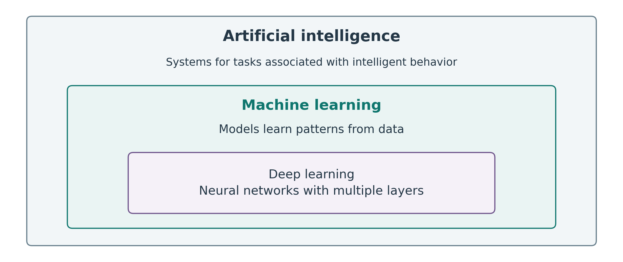
Artificial intelligence is the field of building systems that perform tasks associated with intelligent behavior.

An AI system can make mistakes. Its output needs evaluation in the setting where it will be used.

Capability	Example
Perceive	Identify a defect in an image
Predict	Estimate a machine’s remaining useful life
Reason	Combine facts and rules to assess possible causes
Generate	Produce a candidate design or a draft report
Support decisions	Recommend which equipment to inspect

These capabilities can overlap. A system may interpret an image, predict a defect category, and recommend an inspection. The examples describe tasks, not a claim that every AI system can perform all of them.

AI, Machine Learning, and Deep Learning

Choose the method according to the task, available data, and practical requirements.

AI includes methods based on explicit rules as well as methods that learn from data. Machine learning learns patterns from examples. Deep learning uses neural networks with multiple layers. Deep learning is useful for many tasks, but it is not always the best choice, especially when data or computing resources are limited.

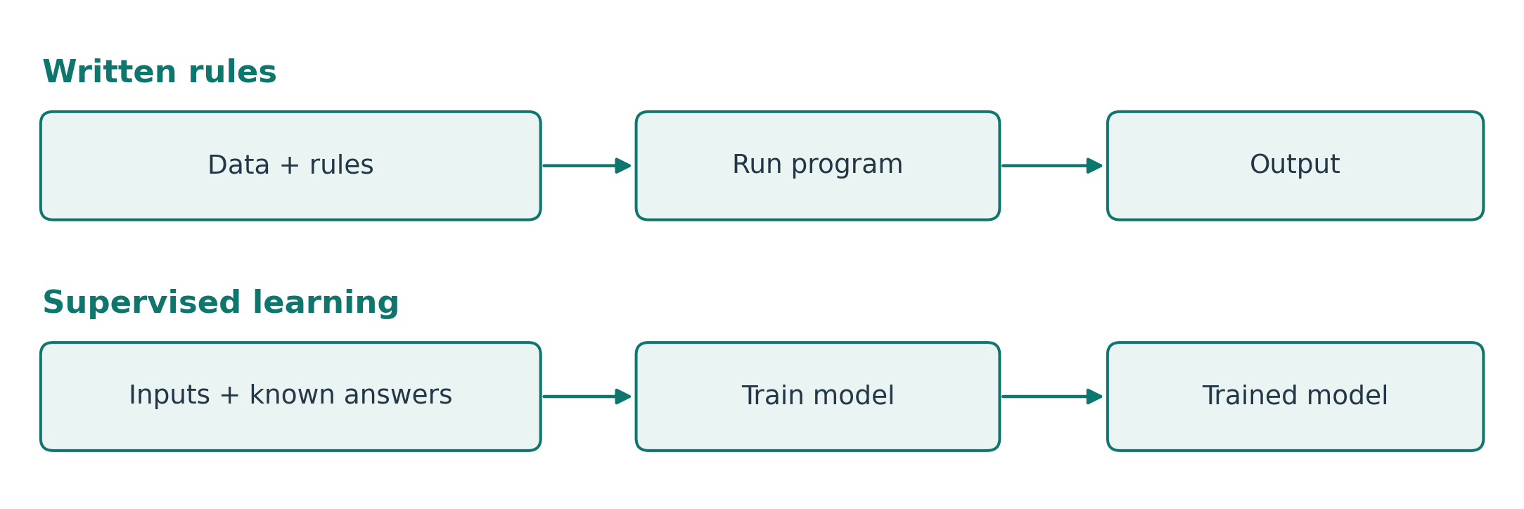
Rules and Learning From Examples

• Written rule: flag a pump when its temperature exceeds a set limit.
• Learned model: use past sensor readings and failure records to estimate failure risk.

This learning example is supervised learning: the training data includes known answers.

A model is a learned relationship between inputs and outputs. It does not necessarily produce readable rules. Other forms of machine learning do not require a known answer for every example. Rules and learned models can also be combined in one application.

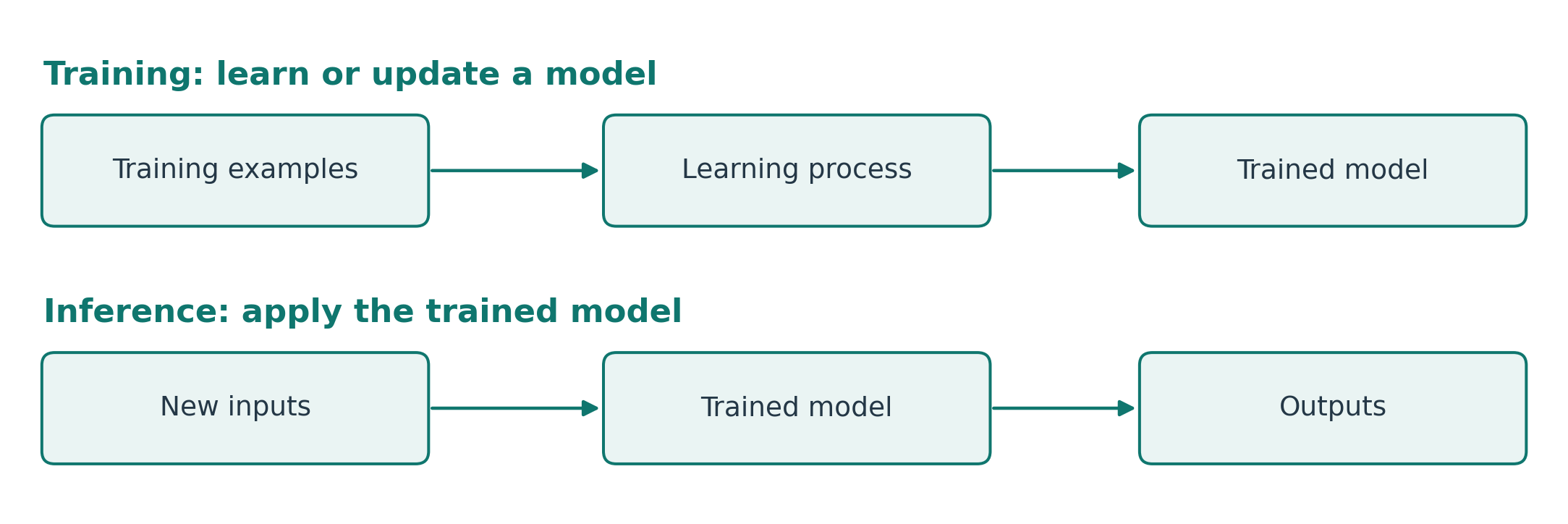
Training and Inference

• Training: learn or update a model from data.
• Inference: apply the trained model to an input.

Models may be retrained. Inference may run immediately or in scheduled batches.

For example, train a pump model using past operation and maintenance records, then use it to estimate risk from recent readings. Neither clean training data nor fast inference is automatic: both require appropriate preparation and engineering.

Common Tasks in Applied AI

One setting—a factory—can involve several tasks:

Task	Purpose	Factory example
Regression	Predict a number	Estimate product strength
Classification	Assign a category	Label a product as defective or acceptable
Forecasting	Predict future values	Estimate next week’s electricity demand
Anomaly detection	Identify unusual patterns	Flag unusual pump vibration
Generation	Produce candidate outputs	Propose a component design
Optimization	Search for the best feasible option	Select operating settings

These categories overlap. Forecasting a number is also regression. Optimization may use an AI model, but optimization itself does not require AI. An anomaly is an unusual observation; it is not automatically a confirmed failure.

Define a Useful AI Task

Start with a practical need: reduce unplanned pump downtime.

A concrete task statement:

Estimate whether a pump will fail within the next 24 hours, using recent sensor readings, so a maintenance planner can prioritize inspections.

This names the output, time horizon, data, and user.

Quick check (1 minute): what task type is this, and what past records would be needed?

Suggested answer: binary classification, because the outcome is failure or no failure within a specified interval. Training needs sensor histories paired with reliable failure times. Inputs must be available when the prediction is made. An alternative task could predict remaining useful life, which is regression.

2. From a Model to a Working System

Connect the Output to a Decision

For the pump example:

• Output: estimated failure risk within 24 hours
• User: maintenance planner
• Action: review the alert and schedule an inspection
• Value: fewer unexpected stops, with a manageable inspection workload

An output can also support understanding, such as a report or an explanation. In each case, identify who uses it and how it helps. A risk estimate alone does not determine the action; the planner also considers inspection capacity and the consequences of a missed failure.

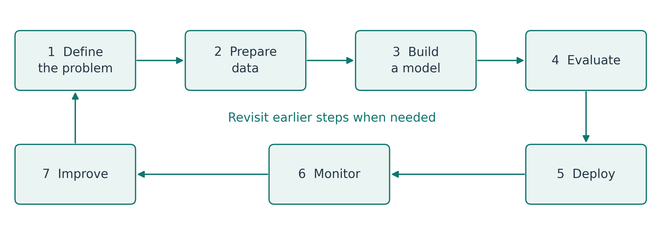
The Applied AI Lifecycle

Deployment puts a model into use. Monitoring checks its behavior after deployment.

Return to earlier steps when the data, requirements, or results change.

Explain each stage using the pump example. Evaluation should precede deployment. Monitoring checks data quality, model performance when outcomes become available, and practical value. Improvement may require changing the data or workflow rather than retraining the model.

What Data Does the Task Need?

Labels are needed for supervised learning. Other learning approaches may use unlabeled data.

Question	Pump example
Features: what inputs are available?	Recent temperature, vibration, and load
Labels: what answers are known?	Whether failure occurred in the next 24 hours
Quality: are records reliable?	Correct timestamps and working sensors
Coverage: what conditions are represented?	Different pumps, loads, and seasons

For historical training examples, derive labels from later failure records. During inference, that future outcome is unknown. Using it as an input would be data leakage: information from outside the valid prediction setting entering the model.

Data Has Different Forms

• Structured data: values organized in fields, such as a table of sensor measurements.
• Unstructured data: content such as images, free text, and audio.
• Sequential data: observations with a meaningful order, such as readings over time or depth.

These descriptions can overlap: a table of hourly readings is both structured and sequential.

The data’s form helps determine how to prepare it and which models to consider.

This distinction prepares students for the two case studies: engineering design records and well measurements ordered by depth. Logs can be structured records or free text, so the word “log” alone does not tell us the data format.

Evaluate the Model and the Application

A baseline is a simple method used as a reference for comparison.

For a pump warning system, check:

1. Prediction quality: how many failures are detected or missed?
2. Comparison: does it improve on a simple temperature rule?
3. Practical use: are warnings early enough and false alarms manageable?
4. New conditions: does it work on data representative of future use?

Use separate data for training, validation (model selection), and testing (final evaluation).

Do not repeatedly tune a model against its final test results. For time-ordered data, use a split that reflects future use. If the aim is to support new machines, test on held-out machines where feasible. These are general evaluation principles, not claims about the exact protocols of the case-study papers.

Why High Accuracy May Be Misleading

Suppose only 5 of 100 examples contain a failure.

A system that always predicts “no failure” has 95% accuracy, but detects none of the failures.

Even a model with useful predictions can fail in practice if:

• its output arrives too late;
• users cannot check or act on the result;
• operating conditions change after deployment.

Choose measures that reflect the purpose of the application.

The numbers are a teaching example. Explain accuracy as the share of correct classifications. Ask students why missed failures and unnecessary inspections should both be measured. Also consider privacy, access permissions, and human oversight when they are relevant to an application.

3a. Case Study: Engineering Design

Agung Nugraha, Hyerin Kwon, Gyeongho Park, and Jihwan Lee (2025). “Cooperative neural networks for inverse design: Integrating denoising autoencoder and surrogate model for partial design variable imputation.” Engineering Applications of Artificial Intelligence, 162, 112453. doi:10.1016/j.engappai.2025.112453.

The Problem: Glass Run Channel Design

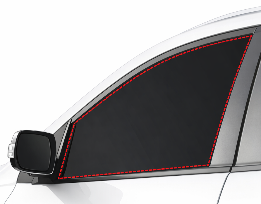
A glass run channel guides and seals a car’s moving window.

• Some design dimensions are already fixed.
• Engineers must choose the remaining dimensions.
• The complete design must satisfy performance requirements.

Task: propose the remaining values while keeping the fixed values unchanged.

Introduce the component before introducing inverse design. The study used an industrial glass run channel case from a Korean automotive manufacturer. A fixed value represents a requirement the method must preserve.

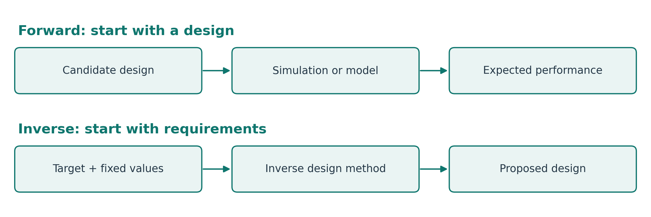
Forward Prediction and Inverse Design

• Forward: what performance will this design produce?
• Inverse: what design could achieve this performance?

An inverse problem can have several solutions—or no feasible solution. A proposed design still needs validation.

A forward relationship cannot always be reversed directly. Inverse design may use generation, optimization, or a learned mapping. “Proposed” matters: a model’s output is a candidate, not a verified physical result.

Partial Inverse Design

Partial inverse design chooses only the free design variables while preserving the fixed ones.

The study treats the free variables as missing values to estimate.

Imputation means estimating missing values from the available information.

Illustrative example:

Given	To be estimated	To be checked
Fixed dimension A and target performance	Free dimensions B and C	Does the complete design satisfy the requirements?

The dimensions A, B, and C are teaching placeholders, not the paper’s named variables. This is intentionally different from repairing a lost measurement: the missing entries represent design choices. The target guides the completion. Detailed probability notation is unnecessary for this overview.

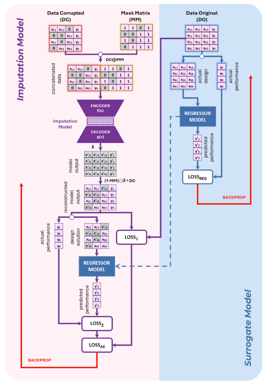
The Approach: Two Cooperating Networks

• Imputation model: proposes the missing design values.
• Surrogate model: estimates performance as a fast substitute for simulation.
• Joint training: uses reconstruction and performance errors to guide learning.

Read the figure in two parts: the imputation model on the left and the surrogate model on the right.

Original manuscript figure: Nugraha et al. (2025).

The imputer uses a denoising autoencoder, a neural network trained to reconstruct incomplete or corrupted inputs. On the left, the mask identifies missing entries, and the encoder and decoder estimate their values. On the right, the surrogate learns from complete designs and their performance values. The loss terms connect reconstruction and performance during joint training; the red arrows indicate backpropagation, which updates model parameters. Introduce the two roles without requiring students to follow every symbol. A surrogate is also an approximation, so its prediction does not prove that a candidate is physically valid.

Engineering Case: Results and Limits

The paper reports, in its initial tests:

• reductions in mean squared error (MSE) of up to 98% relative to compared methods;
• R-squared values of 0.997–0.999.

Interpretation: the approach performed well in the reported experiments. These are not guarantees for new designs.

Potential use: help engineers identify promising candidates before further simulation or physical testing.

Reported results: Nugraha et al. (2025).

MSE averages squared differences between estimated and reference values; lower is better. R-squared compares squared error with a reference that predicts the evaluation-set mean; values closer to one indicate a better fit. R-squared is not a percentage of correct designs. “Up to” describes the largest reported reduction, not every experiment. Do not interpret this number as a measured reduction in prototype cost or design time.

3b. Case Study: Well-Log Reconstruction

Gian Antariksa, Radhi Muammar, Agung Nugraha, and Jihwan Lee (2023). “Deep sequence model-based approach to well log data imputation and petrophysical analysis: A case study on the West Natuna Basin, Indonesia.” Journal of Applied Geophysics, 218, 105213. doi:10.1016/j.jappgeo.2023.105213.

The Problem: Missing Well-Log Measurements

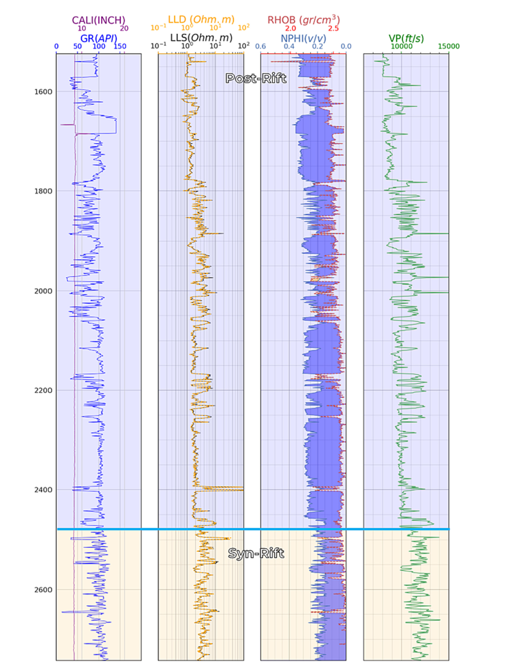
A well log records measurements along the depth of a drilled well.

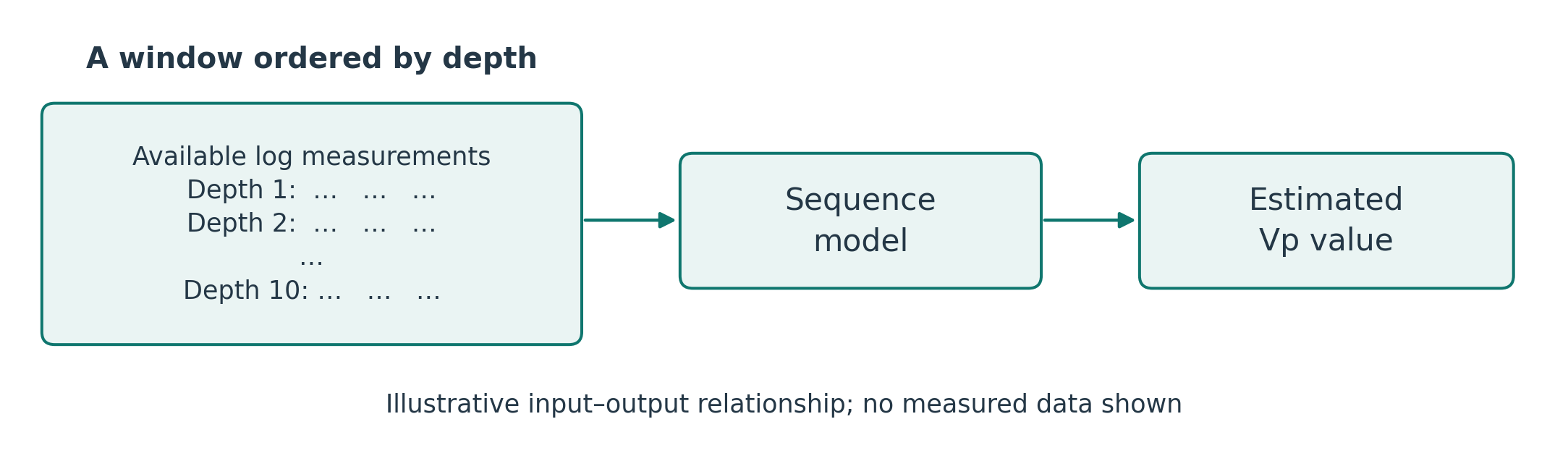
The study estimates missing Vp values: the speed of compressional waves through the rock.

• Input: other available log measurements
• Output: estimated Vp at the required depths
• Use: support interpretation of reservoir properties

Case and figure: Antariksa et al. (2023), West Natuna Basin, Indonesia.

Logging can occur during or after drilling. Missing or unreliable measurements may result from tool or operational problems. Vp means compressional-wave velocity; it is not itself a direct measurement of how much oil is present. Petrophysical analysis uses measurements to estimate rock and fluid properties.

Why Use a Sequence Model?

• Neighboring depths can provide useful context.
• A sequence model learns from ordered observations.
• The study compared LSTM, GRU, and bidirectional LSTM using windows of 10 steps.

Method: Antariksa et al. (2023). Diagram is illustrative.

LSTM means long short-term memory; GRU means gated recurrent unit. Both are neural-network designs for sequences. Bidirectional LSTM processes a sequence in both directions. Here the order is depth, not time. Nearby readings may be related, but rock properties can change abruptly at layer boundaries. Do not assume missing values are always a smooth continuation.

Well-Log Case: Results and Limits

The best reported model was LSTM:

• MAPE about 2.2%: average absolute percentage error
• R-squared about 0.94: a measure of fit to reference values
• The reconstructed logs were used in petrophysical analysis: interpretation of rock and fluid properties.

Limit: these results describe the studied dataset. Performance on another well or geological setting needs separate evaluation.

Reported results: Antariksa et al. (2023).

MAPE expresses each absolute error relative to its reference value and then averages the percentages. It can be misleading when reference values are near zero. A 2.2% average does not mean every estimate is within 2.2%. Evaluate against known measurements held out from training; the true values of genuinely missing measurements are not available for a direct error calculation.