Lecture 2: Special Topics in Machine Learning

ML Strategy, Error Analysis, and Simple ML Serving

Special Topics in Artificial Intelligence (STAI 2026)

Why This Lecture Matters

• Training a model is the easy part. Deciding what to do next is the hard part.
• A typical ML project offers dozens of possible improvements: more data, bigger model, new architecture, more tuning…
• Trying them randomly can waste weeks or months.
• Today: a way of thinking about ML projects, used by experienced practitioners.

Open with a story: a team spends three months collecting more data, and the model barely improves. The problem was not effort, it was direction. This lecture is about choosing direction. Emphasize that this lecture has almost no math on purpose: it is about judgment.

Today’s Roadmap

Part	Topic
1	Why ML strategy, and orthogonalization
2	Setting the goal: metrics and data splits
3	Human-level performance, bias and variance
4	Error analysis and prioritization
5	When training data and real data differ
6	From model to application: simple ML serving

Two hours total. Parts 1 to 5 are adapted from Andrew Ng’s ML Strategy material. Part 6 is new: a gentle, conceptual introduction to serving a model with an API and Docker, with a short live demonstration. Full references are listed on the course website (Week 2 page).

Part 1: Why ML Strategy?

A Familiar Scenario

You built a cat classifier. After some training: 90% accuracy.

Not good enough for your application. What now?

• Collect more data?
• Collect a more diverse training set?
• Train longer? Try a different optimizer?
• Try a bigger network? A smaller network?
• Try dropout? Add regularization?
• Change the architecture?

Ask the class first: what would YOU try? Collect a few answers. The point is that all of these sound reasonable, and that is exactly the problem. Each one can cost weeks. Teams that pick badly can spend six months on something that was never going to help.

Strategy Means Choosing What to Fix First

Key idea

ML strategy is a set of quick, reliable ways to figure out which ideas are worth pursuing and which you can safely discard.

• Without strategy: trial and error, wasted effort, frustration.
• With strategy: measure, diagnose, then act on the bottleneck.
• The rest of this lecture is a toolbox for that diagnosis.

Analogy: a doctor does not prescribe every medicine at once. First diagnose, then treat. We will learn to diagnose ML systems the same way.

Part 1b: Orthogonalization

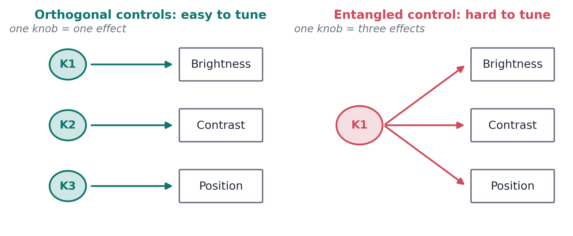
One Knob, One Effect

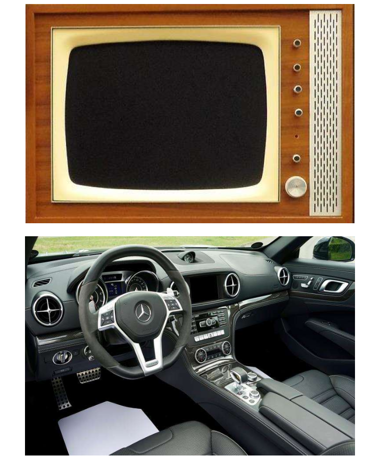
Old TV sets were easy to tune because each knob did one thing. Same in a car: steering for direction, pedals for speed.

Orthogonalization

Design your workflow so that each “knob” fixes one specific problem.

Orthogonal means “at 90 degrees”: each control moves the system along one independent direction. Same in a car: steering for direction, pedals for speed; nobody wants one control that does both. This is why experienced practitioners are calm: when something is wrong, they know exactly which knob to reach for.

The Chain of Assumptions in ML

For a system to work in practice, four things must be true in order:

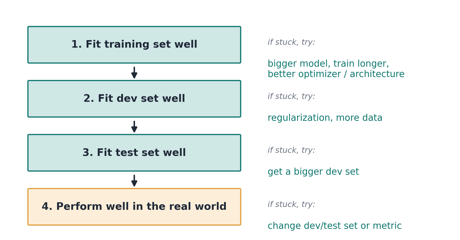
If stage 2 fails, stage 3 knobs will not help.

Walk through the chain slowly, it structures the whole lecture. Dev set = development set, also called validation set: the data we use for choosing between models. Stress the “in order” part: it makes no sense to worry about real-world performance if the model cannot even fit its own training data.

Which Knobs Fix Which Stage

Problem	Typical knobs
Poor fit on training set	Bigger model, train longer, better optimizer, better architecture
Poor fit on dev set	Regularization, more training data
Poor fit on test set	Get a bigger dev set (you over-tuned to it)
Poor real-world performance	Change the dev/test set or the metric (they aim at the wrong target)

Do not explain each technique deeply, that is not the point today. The point is the mapping: problem type to knob family. Mention that this table will make much more sense once we can measure which stage is failing, which is the next part.

Discussion (5 minutes)

Your team’s model fits the training data almost perfectly, but performs poorly on new data.

1. Which stage of the chain is failing?
2. Which knobs would you consider first?
3. Would “train longer” help here? Why or why not?

Answer: stage 2 (dev set). Knobs: regularization, more data. Training longer mostly helps stage 1 and can even make stage 2 worse. Let pairs discuss for 3 minutes, then collect 2 or 3 answers. This is the first Havruta-style pause, around minute 15.

Part 2: Setting the Goal

A Single-Number Evaluation Metric

You compare two classifiers using precision and recall:

Classifier	Precision	Recall	Which is better?
A	95%	90%	?
B	98%	85%	?

Two numbers: no clear winner, slow decisions. Combine them into one number, for example F1 (a balanced combination of precision and recall):

Classifier	F1 score
A	92.4%
B	91.0%

Remind briefly: precision = of the items flagged as cat, how many really are cats; recall = of all real cats, how many we found. F1 is the harmonic mean, 2PR/(P+R), but do not dwell on the formula: the message is “one number makes the decision instant”. Another example from the source: classifiers evaluated across four regions; the average error per classifier makes the best one obvious at a glance.

Why One Number Speeds You Up

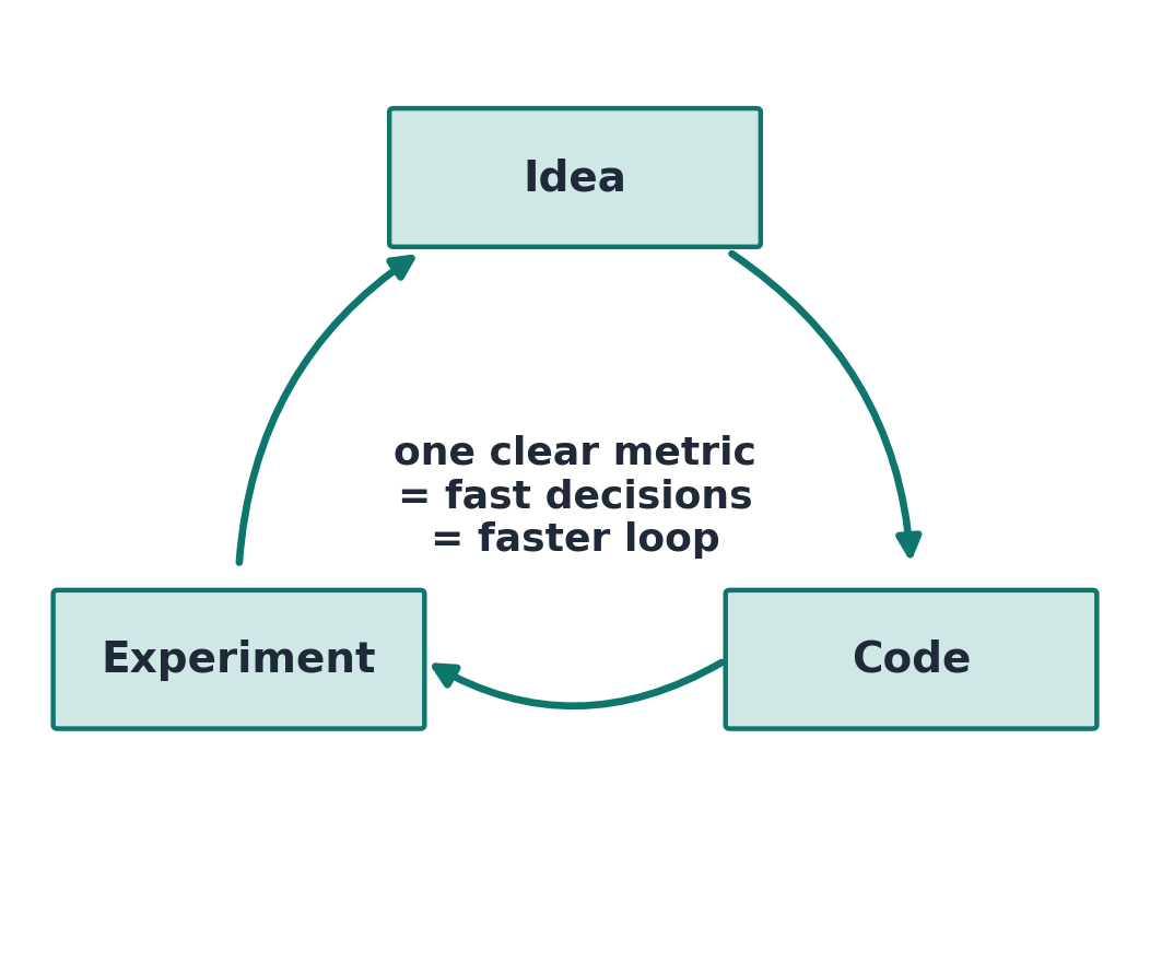
Applied ML is an empirical loop.

• Every experiment ends with a decision: keep it or drop it?
• One clear number makes each decision fast and unambiguous.
• Faster loop = more ideas tested = faster progress.

Teams with a clear metric iterate several times faster, not because they code faster, but because they decide faster. A committee arguing about which of two dashboards of numbers is better can lose a week per decision.

Satisficing and Optimizing Metrics

Not every metric should be maximized. Often you want:

Maximize one metric, subject to constraints on the others.

Classifier	Accuracy	Running time
A	90%	80 ms
B	92%	95 ms
C	95%	1500 ms

Rule: maximize accuracy (optimizing) subject to running time below 100 ms (satisficing). Winner: B.

Satisficing = “good enough is enough”: once running time is under 100 ms, we do not care if it is 95 or 60 ms. Another example: a voice assistant wake word: maximize detection accuracy, subject to at most one false wake-up per 24 hours. General pattern with N metrics: 1 optimizing, N-1 satisficing. Avoid hand-made weighted formulas like accuracy minus 0.5 times time: they are arbitrary and hard to defend.

Guidelines for Choosing Metrics

• Pick one optimizing metric: the thing you truly want more of.
• Turn the rest into thresholds: latency, memory, cost, fairness constraints.
• Write the metric down before running experiments.
• A metric is a target, not a law: if it stops reflecting what you care about, change it (more on this soon).

Quick check (1 minute): for a voice assistant wake word, which metric is optimizing and which is satisficing?

Practical tip for the semester projects: every project report should state its single-number metric and its satisficing constraints explicitly. This one slide will save students a lot of confusion later.

Part 2b: Train, Dev, and Test Sets

What Each Set Is For

Set	Purpose	Used how often?
Training set	Fit the model’s parameters	Constantly
Dev set	Compare models, tune choices	Frequently
Test set	Final, honest performance estimate	Once, at the end

Important

The dev set is the target you aim at for weeks or months. Point it at the right target.

Common student mistake: tuning on the test set. Once you tune on it, it silently becomes a dev set, and you no longer have an honest estimate. Dev set is also called validation set in many textbooks.

Dev and Test Must Aim at the Same Target

Bad idea (true story pattern): dev set from some regions, test set from other regions.

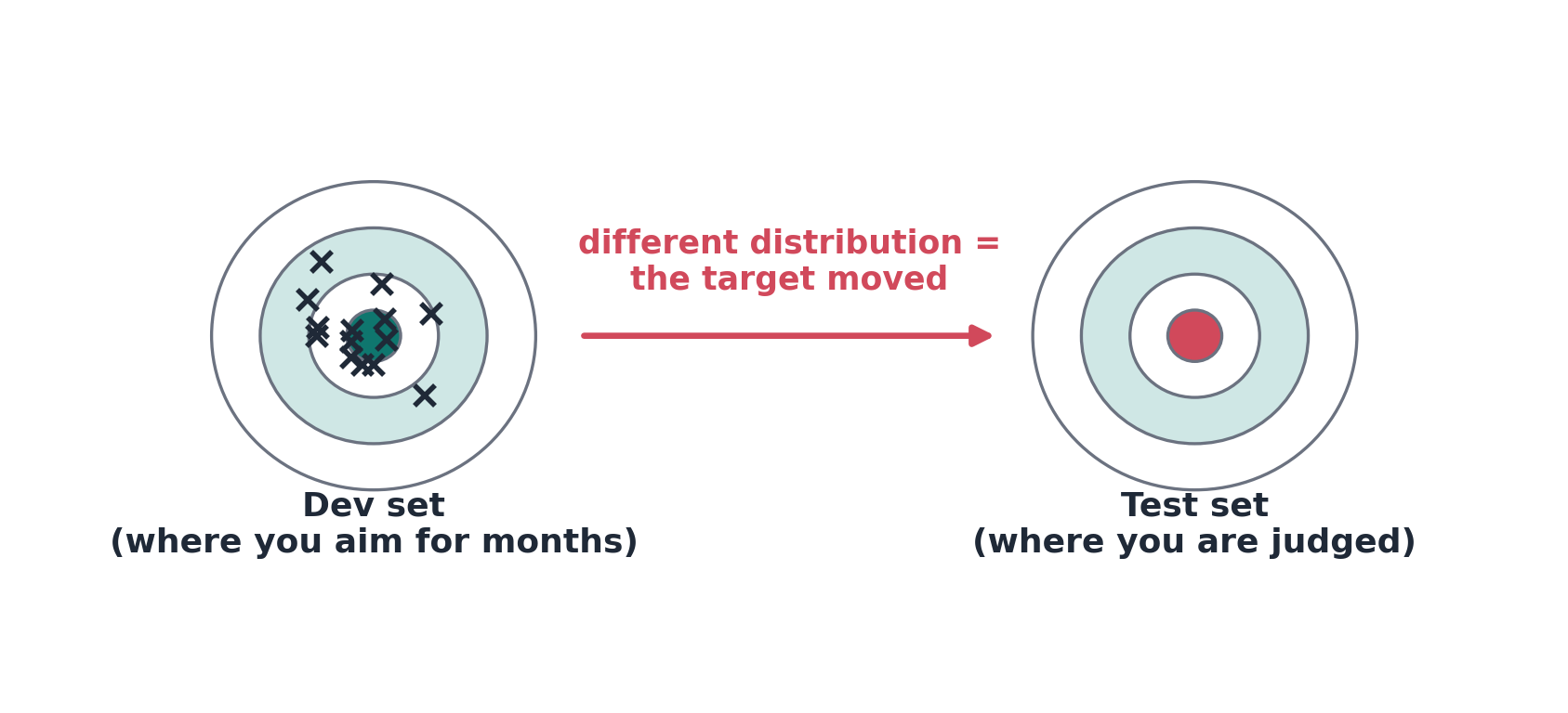
Fix: shuffle everything together, then split dev and test from the same distribution.

Aiming analogy: you practice shooting at one target for months, then someone moves the target on exam day. Real pattern from the source: dev = US, UK, Europe, South America; test = India, China, Asia, Australia. Also mention the loan-approval story: a team optimized on medium-income zip codes and was then evaluated on low-income zip codes; months of work wasted. The guideline slide comes next.

The Golden Guideline

Guideline

Choose dev and test sets that reflect the data you expect to get in the future and consider important to do well on.

• Future user data matters more than convenient historical data.
• If real usage will be blurry phone photos, the dev set should contain blurry phone photos.

This is one of the most quoted lines from the source material, keep it nearly verbatim on purpose (it is a principle, not prose). Everything else in this lecture assumes the dev/test set is pointing at the right target.

How Big Should Dev and Test Sets Be?

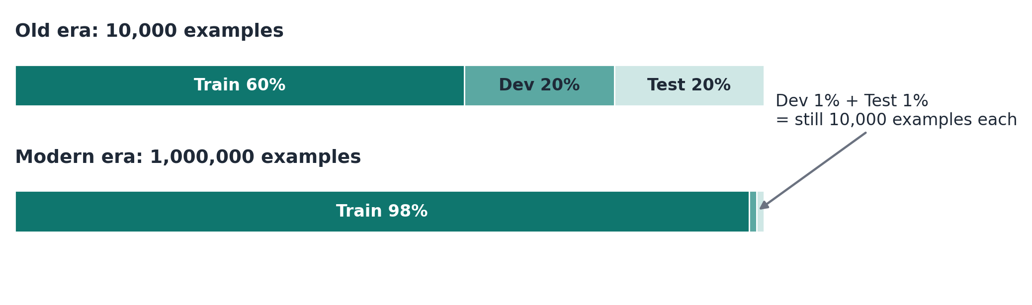
Principle: dev set big enough to detect differences between models; test set big enough for confidence in the final number.

Old rule from the small-data era: 70/30 or 60/20/20. With a million examples, 1% is already 10,000 examples, plenty for evaluation, so 98/1/1 is common. Percentages are not sacred: sizes should follow the purpose of the set. For a class project with 5,000 samples, 60/20/20 is still perfectly sensible.

When Metric and Dev Set Mislead You

• Algorithm A: 3% error, but sometimes shows inappropriate images
• Algorithm B: 5% error, never does

Metric says A; users prefer B. The data can mislead too:

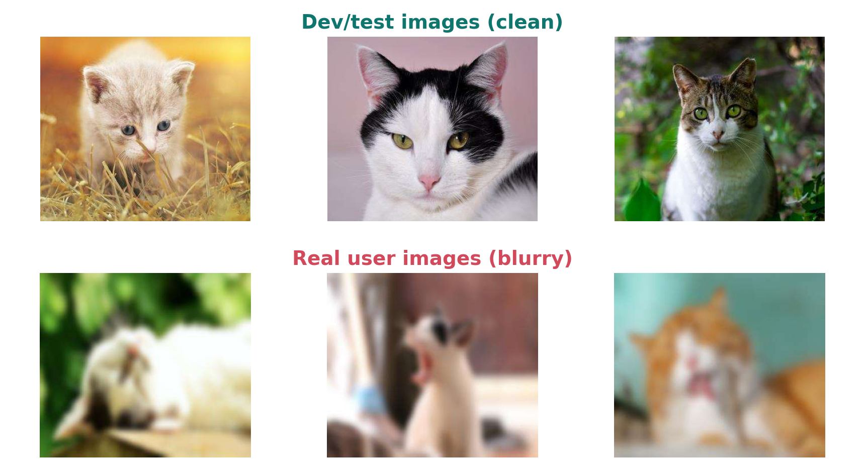
Important

If doing well on your metric + dev/test set does not correspond to doing well in your application: change the metric or the dev/test set.

Two separate failure modes: (1) the metric counts the wrong thing: fix by re-weighting errors, for example penalize unacceptable images much more heavily; (2) the dev set contains the wrong data: fix by rebuilding it from real user images. Do not keep optimizing a target you no longer believe in. This closes the loop with orthogonalization: placing the target and hitting the target are separate knobs.

Discussion (5 minutes)

You are building a defect detector for a factory. You train and evaluate on sharp, well-lit photos from the vendor’s catalog. On the production line, images come from a fixed camera with glare and dust.

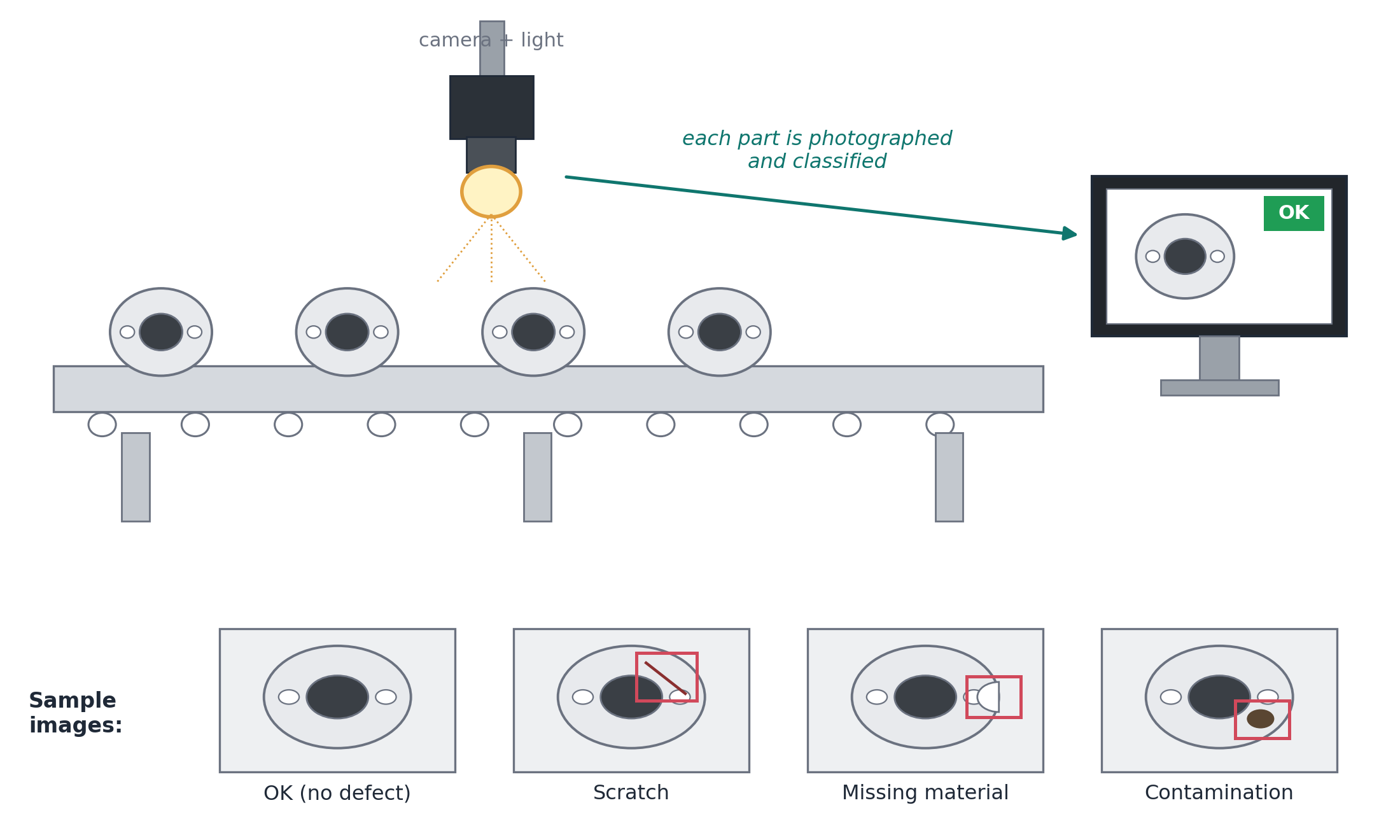
1. What is wrong with the current dev/test setup?
2. What would you change first: the model or the data split?
3. What would your single-number metric be?

Expected conclusions: the dev/test set does not represent future data; fix the target before touching the model; metric could be F1 on defect detection with a satisficing constraint on inspection time per part. Around minute 40. Engineering-flavored example on purpose, closer to the students’ domains than cats.

Part 3: Human-Level Performance

Why Compare With Humans?

While the model is worse than humans, you have tools:

• get more labeled data from humans
• error analysis: “why did a person get this right?”
• better bias/variance diagnosis

Humans are quite good at many tasks (vision, speech, reading). Progress is fast while below human level, then flattens as it approaches the theoretical ceiling: the tools above fade away once you surpass humans. ML already beats humans on some structured-data tasks: online advertising, product recommendations, logistics, loan approvals. Perception tasks are harder to surpass.

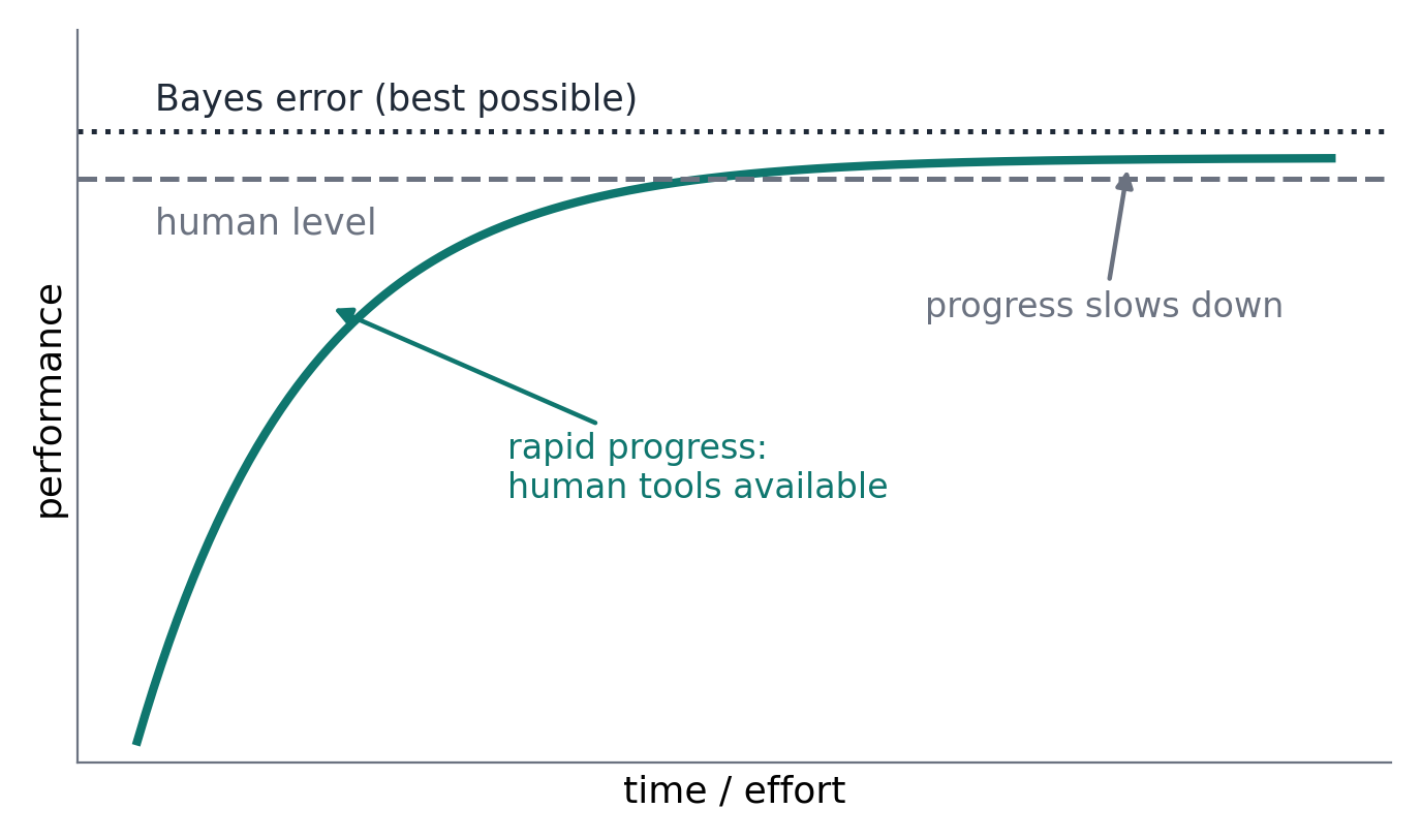
Human-Level Error as a Proxy for Bayes Error

Bayes error: the best possible error any system could ever achieve (some noise is simply irreducible).

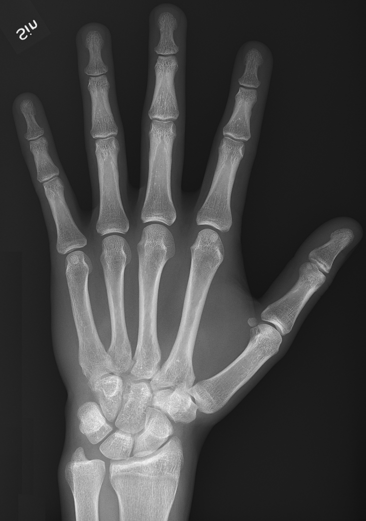
Medical image example: what is “human-level” error?

Who	Error
Typical human	3%
Typical doctor	1%
Experienced doctor	0.7%
Team of experienced doctors	0.5%

Use the best available human performance (0.5%) as the proxy.

Conceptual only, no formulas. Bayes error exists because some cases are genuinely ambiguous (a blurry image nobody can classify). Humans are often close to Bayes error on perception tasks, so “best human error” is a usable stand-in. Which definition of human-level you use depends on the purpose: for deployment maybe “typical doctor” is the bar; for estimating the ceiling, use the best team.

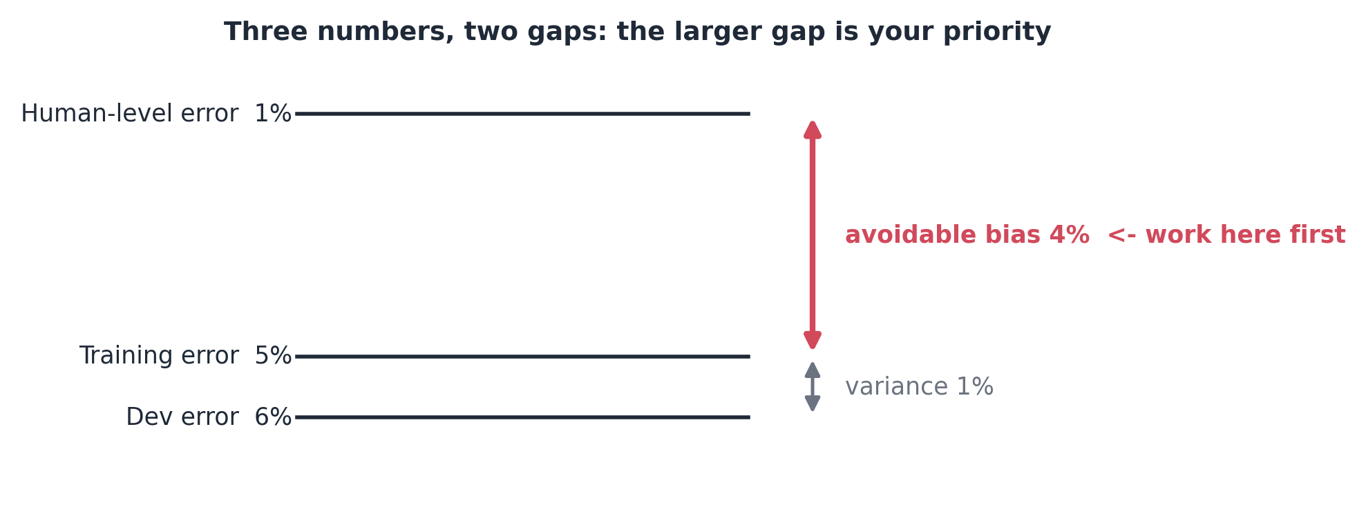
Avoidable Bias

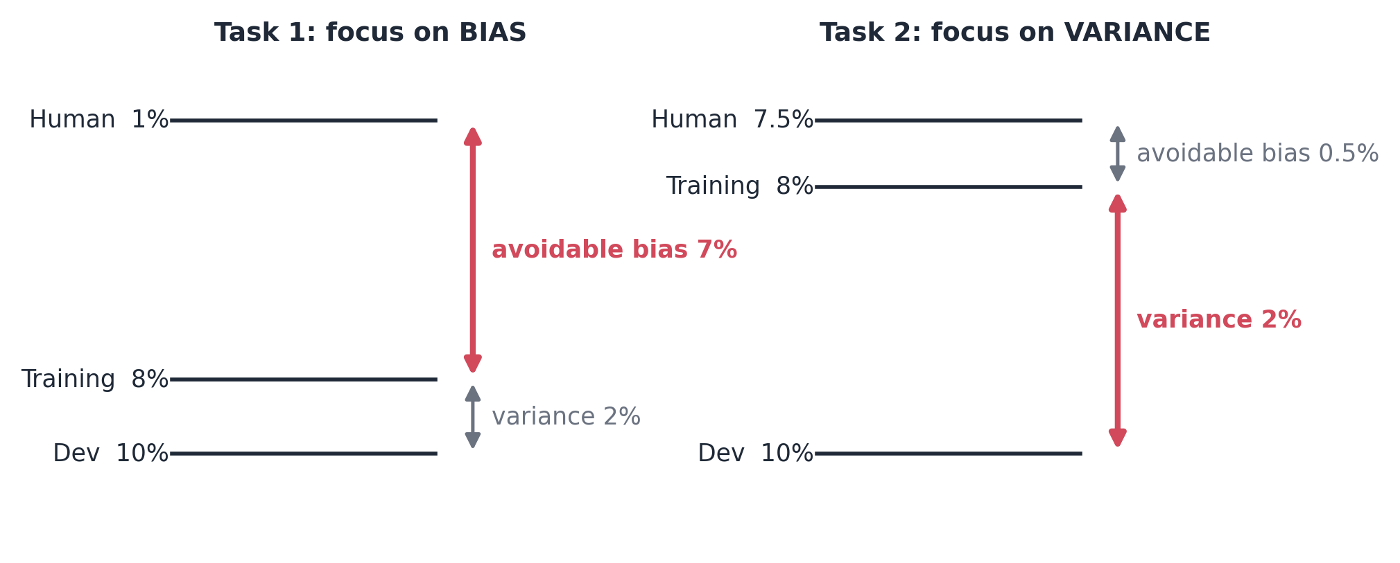
Same training error (8%) and dev error (10%), opposite conclusions:

Task 1: humans get 1%, so the model is far from human level on training data: big avoidable bias, focus on fitting better. Task 2: humans also struggle (7.5%, maybe blurry images), so 8% training error is nearly as good as possible: focus on the variance gap instead. “Avoidable” because you cannot expect to go below Bayes error: the gap between human level and training error is the part you can still fix.

Variance

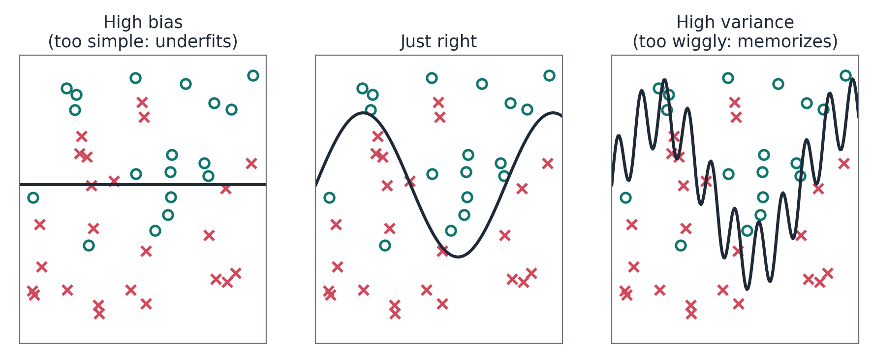
Variance = the gap between training error and dev error: the model memorized more than it generalized.

The classic pictures: an underfitting straight boundary (high bias), a sensible smooth boundary, and a wiggly boundary that traces every noise point (high variance). But the operational definition is just the two gaps: human to training (bias), training to dev (variance). That is what makes it usable day to day.

The Diagnosis Recipe

This one-slide recipe is the heart of Part 3: three error numbers you already have, two subtractions, one decision. In the example: human 1%, training 5%, dev 6%: bias gap 4%, variance gap 1%, so work on bias first. Encourage students to write these three numbers at the top of every experiment log for their projects.

Discussion (5 minutes)

Diagnose each case (human-level error is about 0.5%):

Case	Training error	Dev error	Your diagnosis?
A	6.0%	6.5%	?
B	0.7%	5.0%	?
C	0.7%	0.9%	?

A: avoidable bias problem (5.5% bias gap, 0.5% variance gap). B: variance problem (0.2% vs 4.3%). C: both gaps small: the model is basically done, further tuning has little headroom. Around minute 60, good moment for a 5 minute break after this discussion.

Part 3b: Improving Performance

The Practical Decision Table

Diagnosis	What to try
High avoidable bias (human → training gap)	Bigger model; train longer; better optimizer; better architecture
High variance (training → dev gap)	More data; regularization; data augmentation; simpler model

The two assumptions of supervised learning

1. You can fit the training set well (low avoidable bias).
2. Training performance generalizes to dev/test (low variance).

This table is the payoff of orthogonalization: each row is a stage of the chain, each cell a knob family. Note the tension: a bigger model fights bias but can increase variance; more data fights variance but does not fix bias. That is exactly why you diagnose first. Connect back to the opening scenario: “collect more data” only helps if the problem is variance.

Part 4: Error Analysis

Look at Your Errors. Literally.

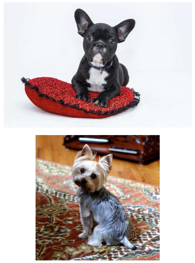
Cat classifier: 10% error. “It keeps mistaking dogs for cats, let’s fix dogs!” Before spending months, do error analysis:

1. Take about 100 misclassified dev set examples.
2. Look at them, one by one, by hand.
3. Count: how many are actually dogs?

• 5 of 100 are dogs: ceiling 10% → 9.5%. Not worth it.
• 50 of 100 are dogs: ceiling 10% → 5%. Very promising.

Students often find “look at 100 images by hand” surprisingly low-tech. Stress: this takes maybe two hours and can save months. The maximum possible improvement from fixing a category is called the ceiling. Two hours of counting versus months of engineering: that is the trade.

Categorize Errors in a Simple Table

Evaluate several improvement ideas in parallel, in a spreadsheet:

Image #	Dog	Great cat (lion, panther…)	Blurry	Comments
1	✓			pitbull
2			✓
3		✓	✓	rainy day at zoo
…
% of total	8%	43%	61%

New categories can be added mid-way (rows can tick several boxes).

The percentages tell you the ceiling for each direction: fixing dogs buys at most 8% relative improvement; blurry images up to 61%. No rigid formula tells you what to do, but the table gives a clear sense of the best options. If halfway through you notice a new pattern (for example filtered images), add a column and keep counting.

Classroom Activity (5 minutes)

Your error analysis of 100 misclassified images gives:

Category	Share of errors
Blurry images	60%
Dogs labeled as cats	25%
Exotic cats	10%
Wrong labels	5%

1. What would you try first, and why?
2. Your teammate insists on fixing the dog problem because it is “technically interesting”. What do you tell them?

Let pairs discuss before showing the next slide, which visualizes the answer. The teammate conversation is the real lesson: interest is not impact; the table is how you keep the discussion objective. Around minute 75.

Debrief: Compare the Ceilings

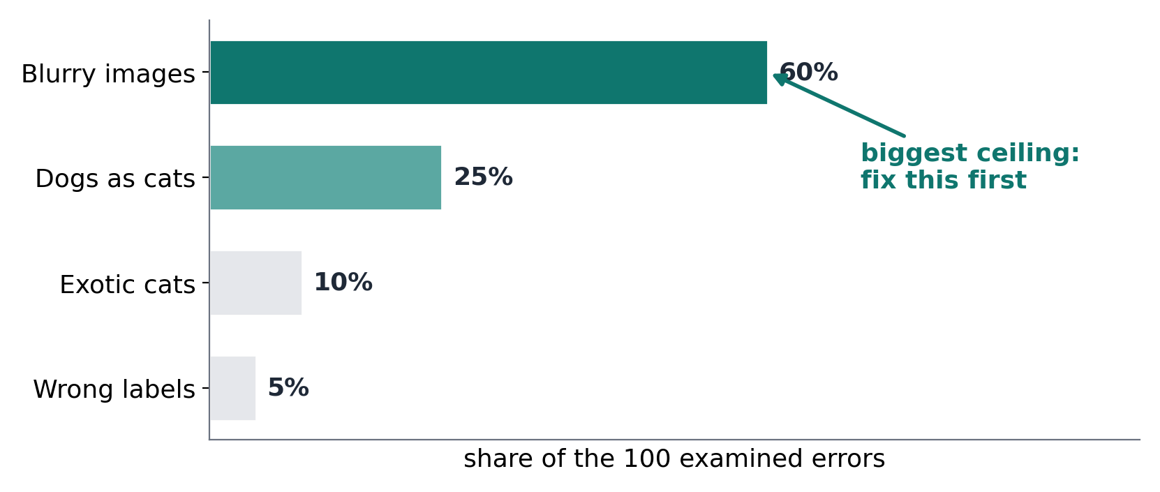
Error analysis does not give a rigid formula. It gives a clear sense of the best options.

Blurry images have a 60% ceiling, by far the biggest. Even a perfect fix of the dog problem caps out at 25%. This chart is what the spreadsheet from two slides ago looks like once you plot the category totals: prioritization becomes visual and hard to argue with.

Incorrect Labels: Training Set

Deep learning is fairly robust to random label errors in training data.

• A few percent of random mislabels: usually fine to leave them.
• But systematic errors are learned! (If white dogs are consistently labeled “cat”, the model will learn it.)

Key nuance: random noise averages out during training, systematic noise becomes a learned rule. So before panicking about a few bad labels in a big training set, ask whether the errors are random or follow a pattern.

Incorrect Labels: Dev and Test Sets

Here wrong labels can corrupt your comparisons between models.

• Add an “incorrectly labeled” column to your error analysis table.
• Dev error 10%, of which 0.6% from bad labels: ignore for now.
• Dev error 2%, of which 0.6% from bad labels: it dominates: fix the labels.

If you clean labels: apply the same process to dev and test, so they stay from the same distribution.

For dev/test the question is: can I still trust that classifier A beats classifier B? Whether 0.6% matters depends on what fraction of the remaining error it is. Also from the source: consider examining examples the model got right, not only its mistakes, and remember cleaning only the dev/test sets means train and dev/test may now differ slightly in distribution, which is usually acceptable but worth knowing. That is the bridge to Part 5.

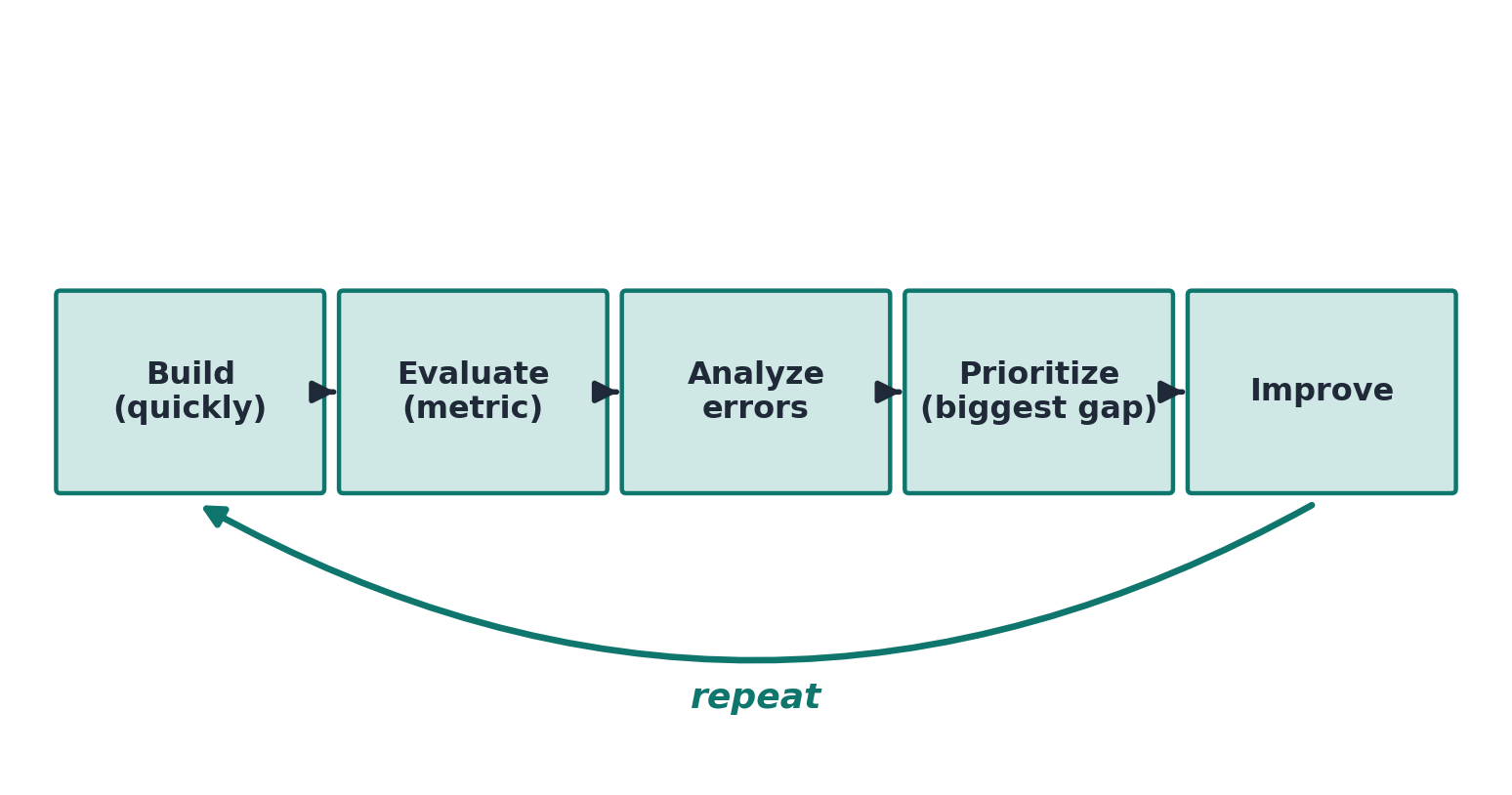
Build First, Then Iterate

Speech recognition: noisy background, accents, far microphone, children, stuttering… Which to focus on? You cannot know in advance.

Guideline: build your first system quickly, then iterate. Set up dev/test and metric, build an initial system fast, then let bias/variance analysis and error analysis tell you what to do next. Do not over-design system number one: its job is to generate errors you can study. A working simple baseline in week 1 beats a perfect design still on the whiteboard in month 3. This loop is literally the recommended workflow for the semester projects.

Part 5: When Training and Real Data Differ

Data Mismatch Is the Normal Case

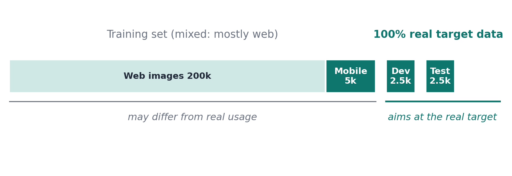
Cat app: 200,000 clean web images available, but users upload 10,000 blurry mobile images. Where should the scarce real data go?

Deep learning is data-hungry, so teams grab whatever data they can: web scrapes, purchased datasets. The tempting alternative, shuffle everything together, is worse: the dev set would then be about 95% web images and you would aim at the wrong target again. The rule from Part 2 wins: dev/test must reflect future real data, even if the training set then comes from a different distribution. Same pattern for speech in cars: purchased clean audio for training, real in-car recordings reserved for dev/test. The next slides show how to measure the cost of that mismatch.

A New Suspect Needs a New Test: the Training-Dev Set

With mismatched data, a train → dev gap has two possible causes:

1. The model does not generalize (variance), or
2. The dev data is simply different and harder (mismatch).

To separate them, carve out a training-dev set:

• same distribution as training data
• not used for training

Now: train vs training-dev isolates variance; training-dev vs dev isolates mismatch.

This is the one genuinely new tool in Part 5. Analogy: two thermometers to find where the heat is lost. Same distribution as training but unseen: so if the model stumbles there, it is a generalization problem; if it only stumbles on dev, the data itself changed.

Reading the Four Gaps

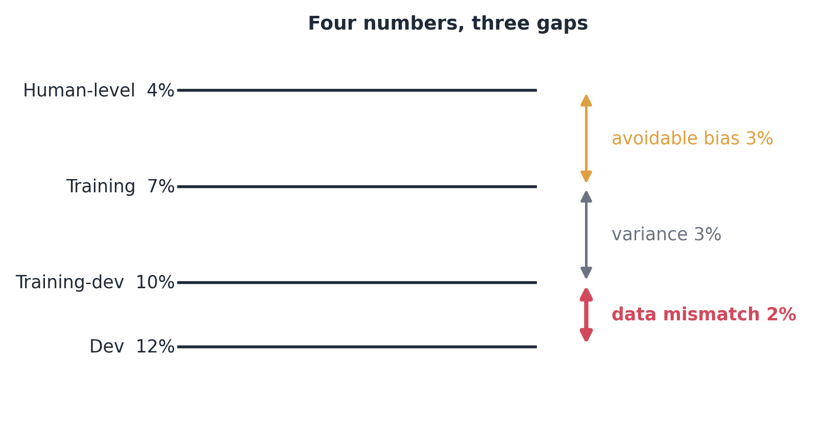
Quick cases (human ≈ 0%):

• train 1%, train-dev 9%, dev 10%: variance
• train 1%, train-dev 1.5%, dev 10%: mismatch
• train 10%, train-dev 11%, dev 12%: avoidable bias

Same recipe as Part 3, just with one more rung on the ladder. Let students diagnose the three quick cases themselves before revealing: it takes 30 seconds each and cements the pattern. Occasionally dev error is lower than training-dev error: that happens when the target data is actually easier, and it is fine.

Addressing Data Mismatch

• Manual error analysis: how exactly does dev data differ? (noise? blur? vocabulary?)
• Make training data more similar to dev/test, or collect more real target data.
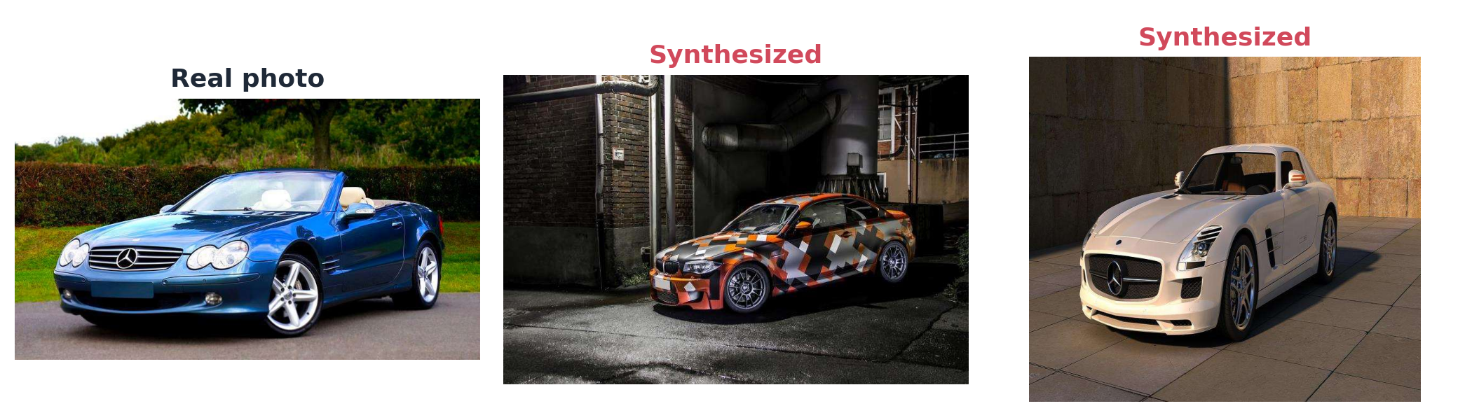
• Artificial data synthesis: clean speech + car noise = in-car audio; rendered objects for images:

Synthesis risk

Synthesizing from a small slice (one hour of car noise, a few 3D car models) makes the model overfit to that slice: perfect to human eyes, yet unrepresentative of the real world.

There is no fully systematic fix for mismatch, these are the practical tools that help. Synthesis is powerful and dangerous: to a human ear the 10,000 hours all sound fine, but the model can memorize the single hour of noise. If you synthesize, maximize the diversity of the ingredients.

Discussion (5 minutes)

A team trains a vibration-anomaly detector for pumps using data from a clean laboratory test rig. Deployed in the plant, it misses real faults.

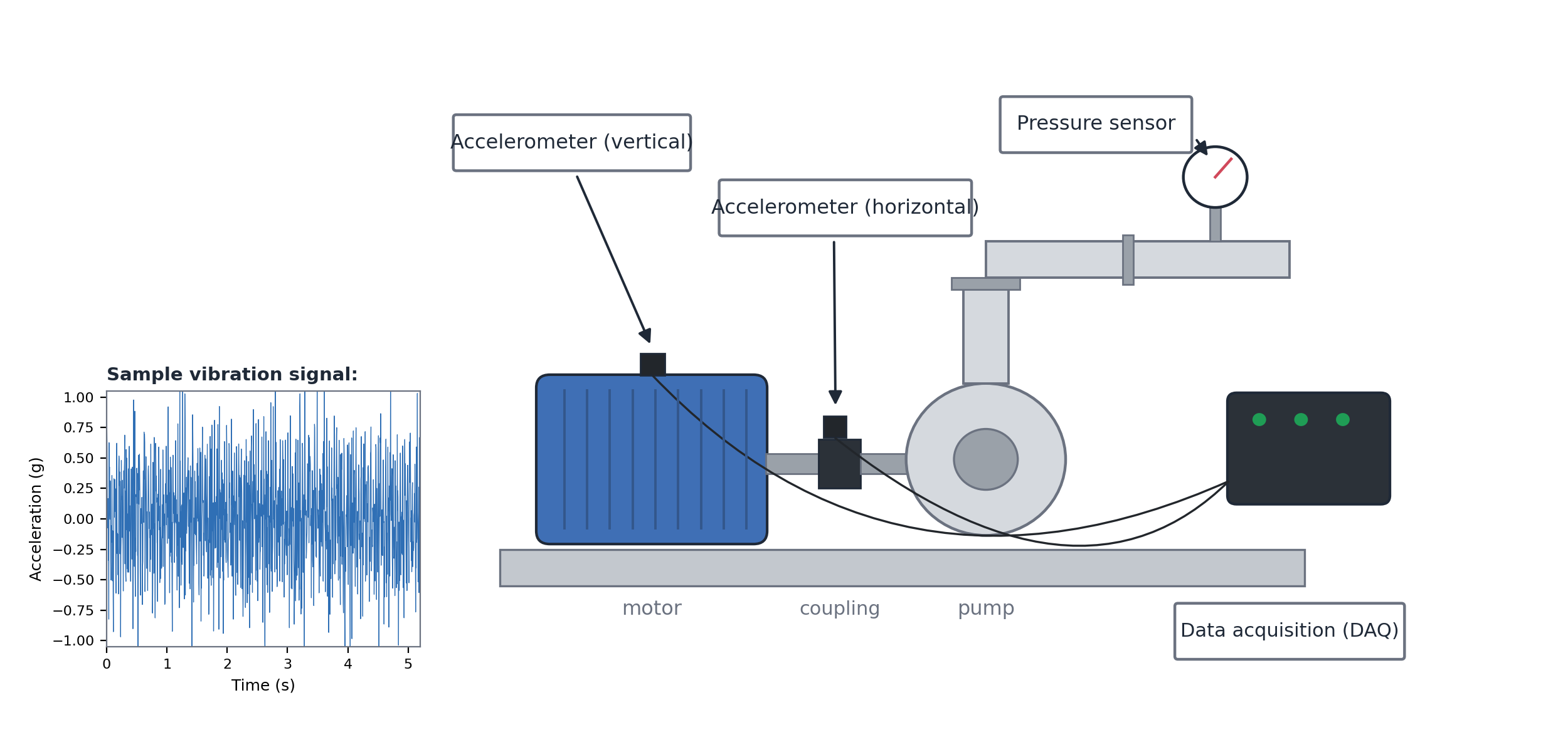
1. Which diagnosis would you check first: bias, variance, or mismatch, and how?
2. The team proposes adding synthetic factory noise to lab signals. What is the promise, and what is the risk?

Expected: build a training-dev split from lab data and compare gaps; if training-dev is fine but plant data fails, it is mismatch. Synthetic noise helps if the noise library is diverse; risk is overfitting to a narrow noise sample. Around minute 95. Last discussion before the serving section.

Part 6: From Model to Application

Training Is Not the End

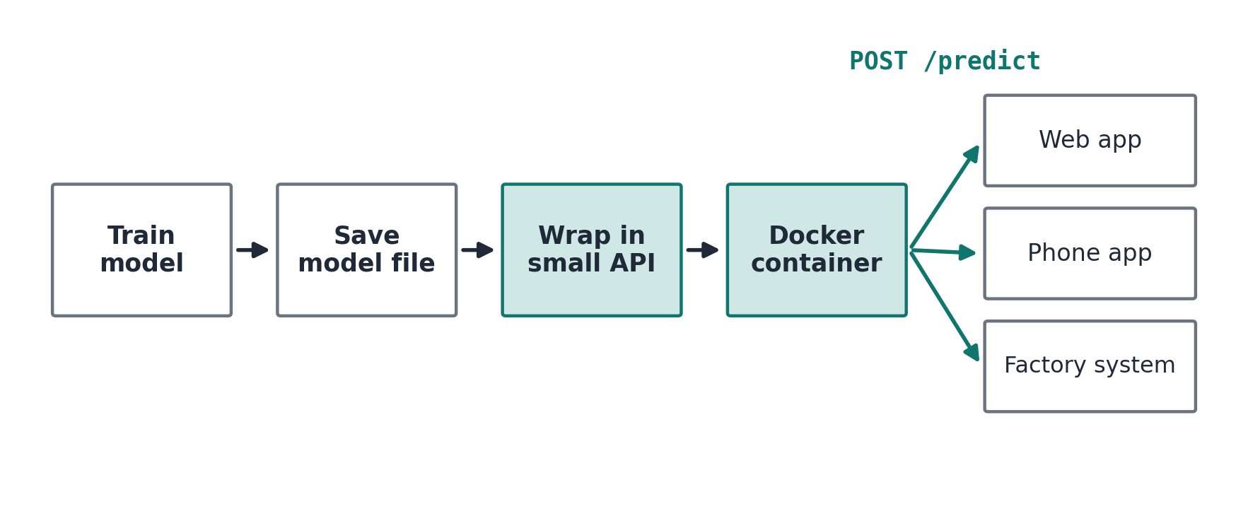
A model in a notebook helps nobody but you. It becomes useful when other people or systems can send it inputs and get predictions back.

ML serving = making your model available as a service:

Deliberate change of altitude: after 90 minutes of strategy, ten minutes of “how does this reach the real world”. The six steps: train, save the model file, wrap it in a small API, put the API in a Docker container, run the container, send input and receive predictions. Keep it light: the goal is the mental model, not DevOps skills. This connects to the semester project: a demo others can actually call is far more convincing than a notebook screenshot.

What Is an API?

API = a defined way for programs to talk to each other over the network.

Your model’s API can be one single “door”:

POST /predict
  input:  { "features": [5.1, 3.5, 1.4, 0.2] }
  output: { "prediction": "class_A", "probability": 0.97 }

• The caller does not need Python, or your libraries, or your GPU.
• A web app, a phone app, or a factory system can all call the same door.

Analogy: a restaurant menu. The kitchen (model) is hidden; the menu (API) defines exactly what you can order and what you get back. POST /predict is the standard idiom: send data, receive a prediction as JSON.

A Tiny Prediction API (Conceptual)

from fastapi import FastAPI
import joblib

app = FastAPI()
model = joblib.load("model.pkl")     # step 2: the saved model file

@app.post("/predict")
def predict(features: list[float]):
    prediction = model.predict([features])
    return {"prediction": prediction[0]}

About 10 lines: your model is now a web service.

Read it top to bottom, do not dissect syntax: load the saved model once, define one function for the /predict door, return the answer. FastAPI turns that function into a real HTTP endpoint. Students will get a working template in the practical materials; nobody is expected to write this from memory today.

What Is Docker?

Problem: “it works on my machine” (but not on the server, or your teammate’s laptop).

Docker packages your code plus its whole environment into one shippable unit:

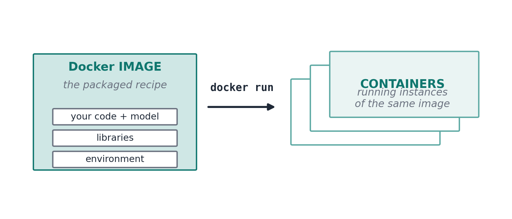
• Same environment everywhere: laptop, server, cloud
• Easy sharing and easy deployment: one command to run

Image versus container is the one distinction worth memorizing: image = recipe or frozen box (code + libraries + environment), container = the running app; you can start many containers from one image. Do not go into Dockerfiles, volumes, or networking: idea only.

Demo: Two Commands

# Build the image (package the app + model + environment)
docker build -t ml-api .

# Run it as a container, exposed on port 8000
docker run -p 8000:8000 ml-api

Then, from anywhere that can reach the machine:

POST http://localhost:8000/predict  →  { "prediction": ... }

Note

You do not need to master Docker in this course. You only need the idea: model → API → container → anyone can use it. We will revisit this hands-on in the practical weeks.

Live demo here if the classroom setup allows (about 5 minutes): build, run, then send one request with the docs page FastAPI generates automatically at /docs. If the demo gods are unkind, walking through these two commands on the slide is enough. Reassure: this becomes a guided exercise later, today is exposure only.

Wrap-Up

Key Takeaways

1. Good ML work needs strategy, not random trial and error.
2. Choose one clear metric and a dev/test set that represents real future data.
3. Diagnose before treating: avoidable bias, variance, data mismatch (three or four numbers, simple gaps).
4. Error analysis: look at about 100 errors by hand, count categories, fix the biggest ceiling first.
5. Build a simple system first, then iterate: Build → Evaluate → Analyze → Prioritize → Improve.
6. A model becomes useful when it is served: API + Docker connect models to real applications.

Close the loop with the opening scenario: the team that “just collected more data” for three months. With today’s toolbox they would have spent one afternoon diagnosing first. If students remember only one slide, it is this one. Full references for this lecture are on the course website, Week 2 page.