Lecture 3: Deep Learning for Structured and Engineering Data

From prediction to representations and modern modeling paradigms

Special Topics in Artificial Intelligence (STAI 2026)

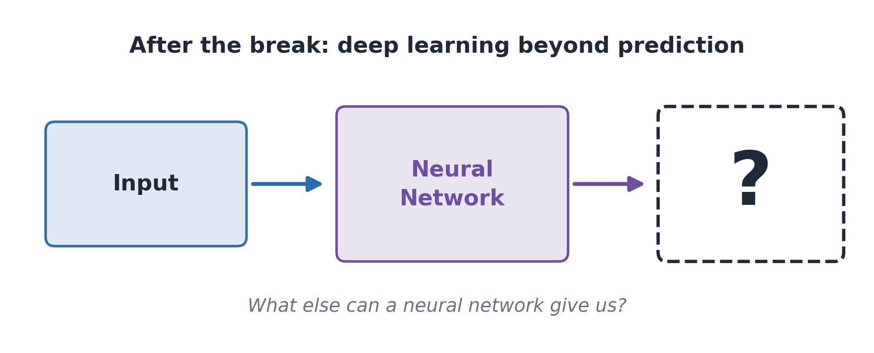
Three Questions for This Lecture

Today we ask three questions about neural networks:

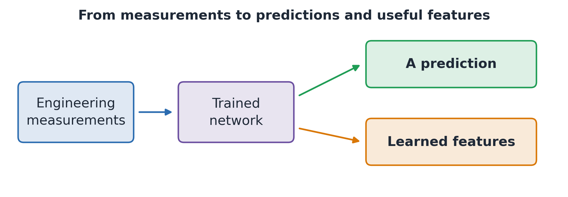
• What can they predict? For example, concrete strength from its ingredients.
• What can they learn from measurements? For example, useful features for detecting machine faults.
• How can several sites learn together? For example, factories training a shared model while keeping their data locally.

FIG. From Measurements to Predictions and Features

Use the three questions to introduce the lecture. A prediction is an estimated outcome, such as compressive strength. A feature is a variable used by a model; a learned feature may summarize a pattern across several measurements. Later examples show how several factories can train a shared model without moving all their raw data to one place. Explain that these are different questions about the use and training of a model.

Today’s Roadmap

Week 2 covered model evaluation. Today we focus on:

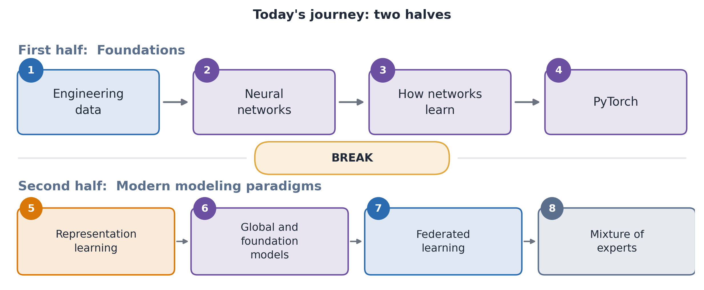
1. Neural-network foundations: how networks make predictions, learn, and are expressed in PyTorch.
2. Engineering applications: how the available data affect our modeling choices.

FIG. Lecture Topics Before and After the Break

Introduce the two halves of the lecture. First, students learn what the network computes and how training changes it. Second, they consider different engineering situations, such as scarce labels, related machines, and data held at different sites. PyTorch is included to connect the concepts to recognizable code. No particular format for a later practical session is assumed.

Engineering Data: Inputs and Targets

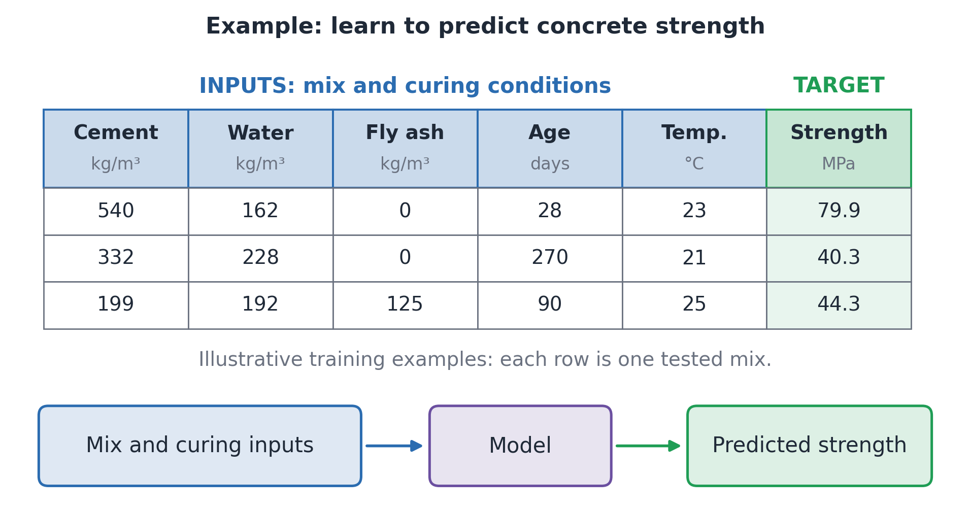
Tabular data are organized into rows and columns.

• Each row is one example, such as a concrete mix tested in a laboratory.
• The inputs describe that mix and its curing conditions.
• The target is measured strength. Use only inputs available for a new mix.

TABLE. Concrete Inputs and Targets

FIG. Predicting Strength

Read one row of the table with the class. Cement, water, fly ash, age, and temperature are inputs. Measured strength is the target available during training. For a new mix, the model receives the inputs and estimates strength; the measured target is not an input. Define a sample as one row and a feature as one input variable. These tabular examples are the focus here, so no comparison with pixels or text tokens is needed.

Typical Engineering AI Problems

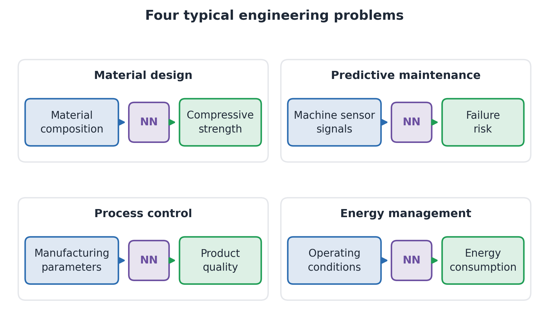
FIG. Engineering Inputs and Prediction Targets

In each example, a model uses measured inputs to estimate an outcome.

Start with a simple comparison model. On small tabular datasets, a random forest or gradient-boosted model may work as well as, or better than, a neural network.

Neural networks are useful when learning features from complex measurements or reusing learning across tasks.

Ask students to identify the input and target in each example. Strength and energy are numerical targets, so these are regression tasks. Fault detection is a classification task. A baseline is a simpler model used for comparison. Deep learning is a choice to evaluate, not an automatic improvement. Keep the concrete-strength example in mind as the network is introduced.

Neural Networks

This section explains the parts of a neural network before discussing training. Begin with a weighted sum, then introduce activation functions, hidden layers, and learned parameters.

From Linear Model to Artificial Neuron

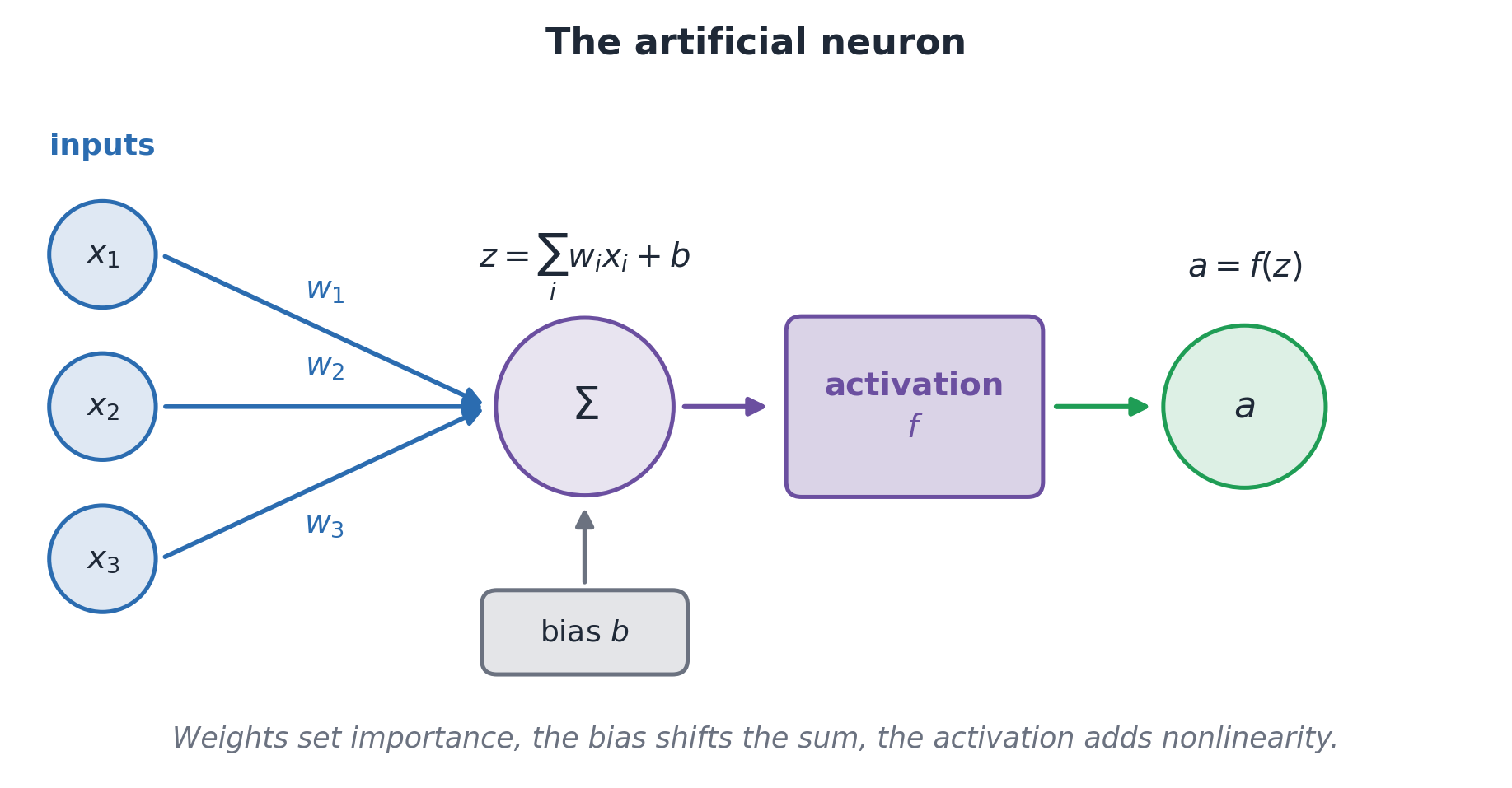
A neuron is a network’s basic building block: it combines inputs, then applies an activation. Training learns how to combine the inputs.

z = w_1x_1 + w_2x_2 + \dots + w_nx_n + b,\qquad a=f(z)

• x_i: input i; w_i: its learned weight; b: a learned bias.
• z: the weighted sum; f: activation function; a: neuron output.

FIG. Weighted Inputs, Bias, Activation, and Neuron Output

The inputs x_i are measured variables. Each weight scales one input, and the bias shifts the sum. The activation function determines how the neuron responds to that sum. A nonlinear activation lets a network describe relationships beyond a linear combination of the original inputs. A linear model can also use engineered nonlinear features, so the comparison here concerns the untransformed inputs. Weight magnitudes alone are not reliable measures of importance, especially when input scales differ.

What Do Hidden Layers Learn?

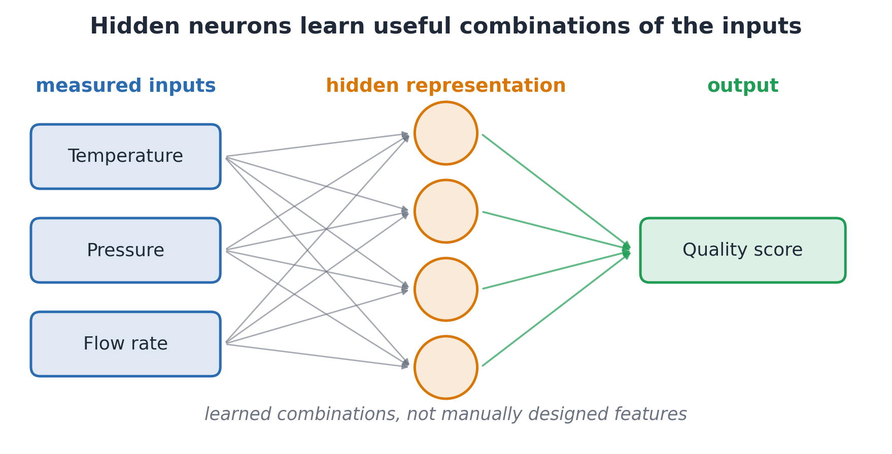
A hidden layer sits between the inputs and the final prediction.

Its units learn combinations of measurements that help the prediction task. For example, a useful combination might involve temperature, pressure, and flow.

FIG. Inputs, Learned Hidden Features, and Prediction

These features form a representation. They help the final layer predict from patterns across measurements. They need not correspond to named physical quantities.

The engineer chooses the network structure, but training learns the weights used to combine inputs. A hidden feature can respond to a pattern across several measurements. It may be useful without corresponding to a familiar quantity such as heat load. Representation learning is the process of learning these useful features. Later, we also consider learning features when task labels are scarce.

From a Neuron to a Network

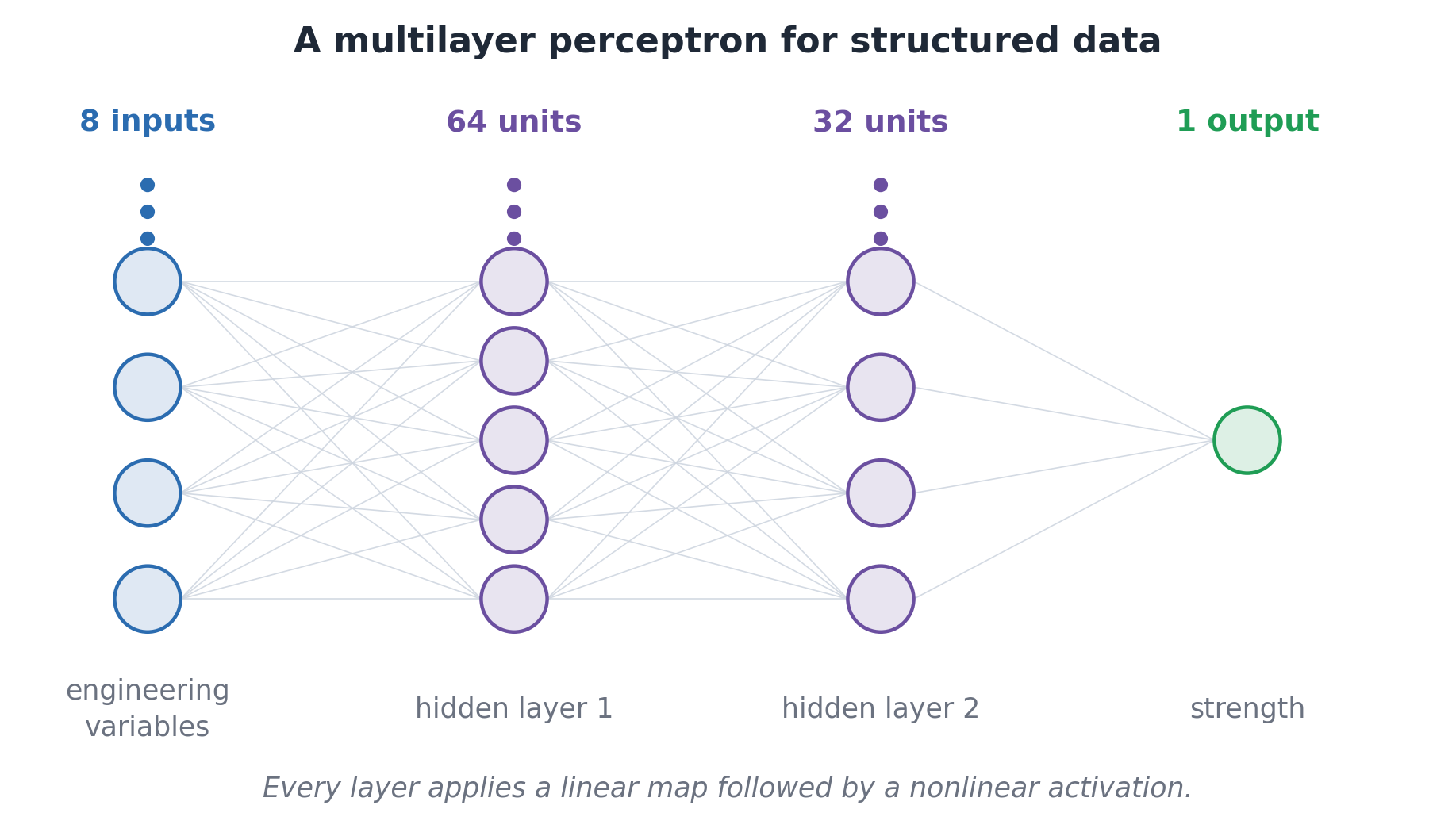
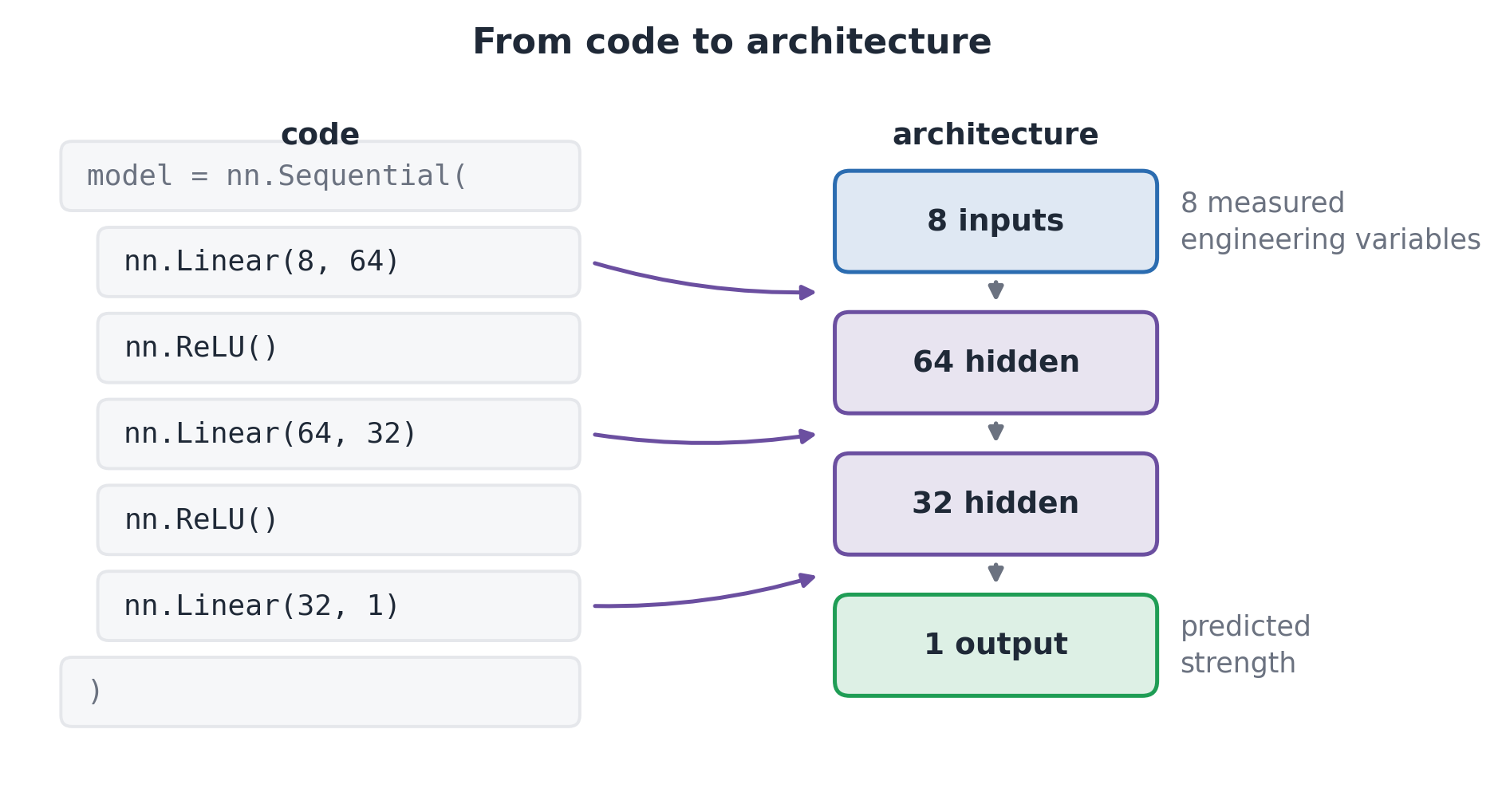
A multilayer perceptron (MLP) is a network of fully connected layers: each unit receives the outputs of the previous layer.

FIG. An Eight-Input Multilayer Perceptron

One layer computes h=f(Wx+b): W contains its weights, b its biases, and h its outputs.

Layers turn measurements into learned features, then a prediction. For example: 8 inputs → 64 units → 32 units → 1 strength prediction.

Explain that W is a matrix containing the weights for a layer, b contains its biases, and h contains its outputs. The hidden-layer widths 64 and 32 are illustrative choices. Deep learning uses networks with multiple learned layers; greater depth does not guarantee better predictions. This is a larger illustrative input set than the five-column dataset shown earlier. An MLP is one common neural-network starting point for tabular data.

Why Activation Functions?

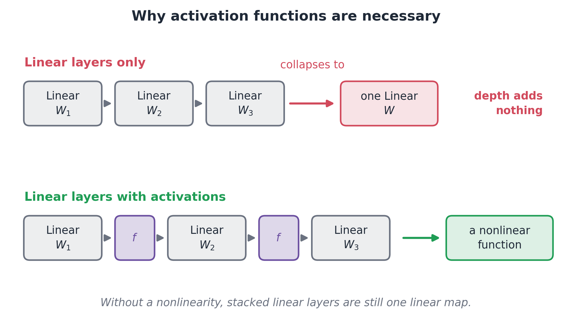
Nonlinear activations let a network learn curved and more complex relationships.

Without them, several linear layers are equivalent to one linear layer:

FIG. Why Stacked Linear Layers Need Nonlinear Activations

Common choices: ReLU for hidden layers; sigmoid for a binary probability; softmax for probabilities across classes. A numerical output often uses no final activation.

For linear layers without biases, multiplying their weight matrices gives one equivalent matrix. Including biases still gives one affine map. ReLU returns max(0,z), sigmoid maps a score into zero to one, and softmax maps a vector of scores to probabilities that sum to one. These are common choices, not universal rules. An unconstrained regression output can take any real value; physical limits may require an additional output transformation.

A Network Maps Inputs to Predictions

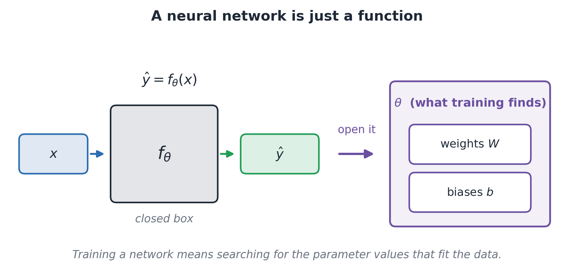
We can write a network’s prediction as \hat{y}=f_\theta(x).

• x: the measured inputs.
• \theta: all the weights and biases that training can change.
• \hat{y}: the predicted output.

FIG. The Network Function and Its Learned Parameters

Training adjusts parameters to reduce prediction errors.

Distinguish architecture from parameters. The architecture specifies which computations are connected; the parameters determine the numerical result. A network stores learned parameters, but those parameters can still memorize training examples. This function notation will be reused when a network is an encoder, a federated model, or an expert.

Part II. How Does the Network Learn?

Make a prediction, measure its error, and update the parameters.

The next section explains training as a repeated process. Students should be able to describe the purpose of each step before worrying about implementation details.

The Forward Pass and the Loss

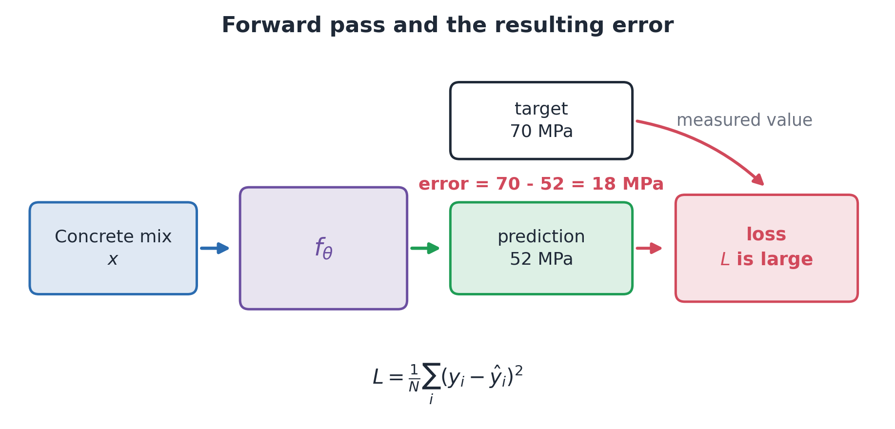
The forward pass computes a prediction. The loss gives training an objective: reduce prediction error.

For N examples, mean squared error compares targets y_i with predictions \hat y_i:

L=\frac{1}{N}\sum_i(y_i-\hat{y}_i)^2

FIG. Comparing Predicted and Measured Strength

Example: 70 MPa measured, 52 MPa predicted. Error magnitude: 18 MPa.

Explain that y_i is the measured target and y-hat_i is the prediction for example i. For the single displayed example, squared error is 18 squared, or 324 MPa squared. Mean squared error averages squared errors over examples. The forward pass does not update parameters. Classification commonly uses cross-entropy loss. Discussion question: why do we usually optimize a smooth loss rather than accuracy? Accuracy changes only when a predicted class changes, so it does not provide a useful gradient for ordinary gradient-based training.

Gradients and Gradient Descent

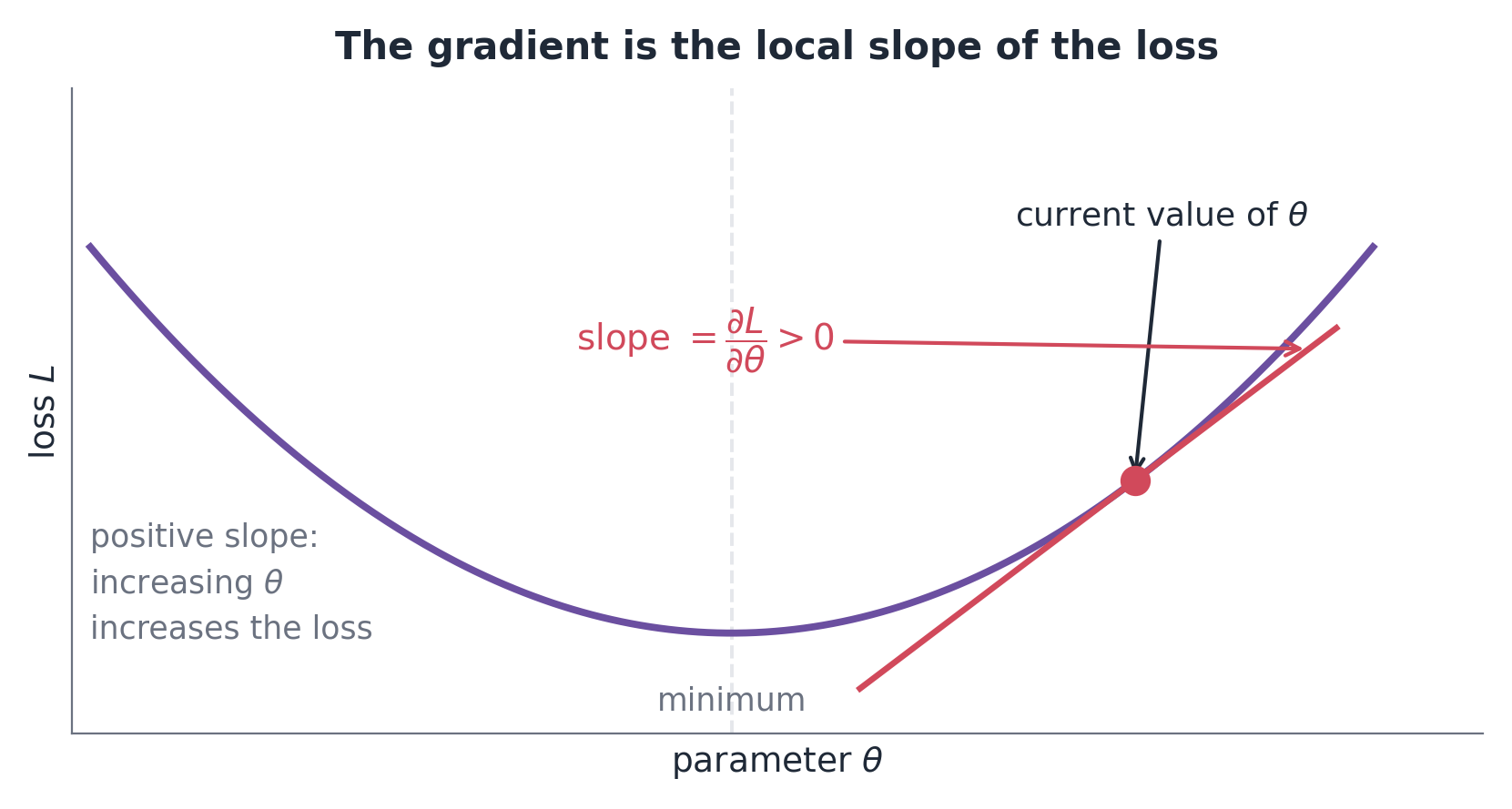
A gradient describes how the loss changes when each parameter changes slightly.

FIG. How Loss Changes with a Model Parameter

Use the gradient to choose an update that aims to lower the loss:

\theta \leftarrow \theta-\eta\nabla_\theta L

\nabla_\theta L is the gradient of the loss. The learning rate \eta controls the update size.

Use the one-parameter curve before discussing a vector of parameters. If the slope is positive, a small move left reduces the loss locally. The gradient contains this local sensitivity for every parameter. It does not identify the global minimum or guarantee that a large step will improve the loss. An unsuitable learning rate can cause slow progress or unstable training.

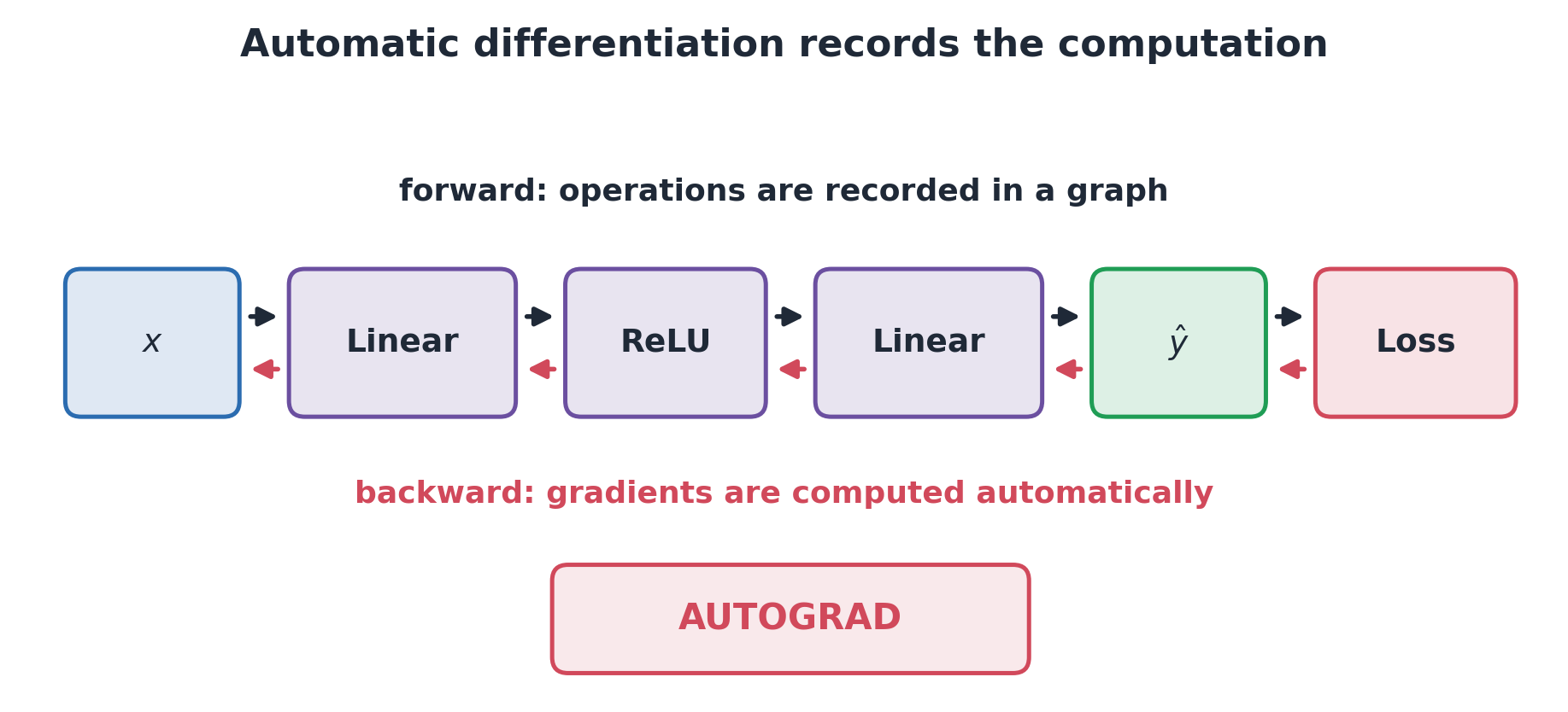
Backpropagation

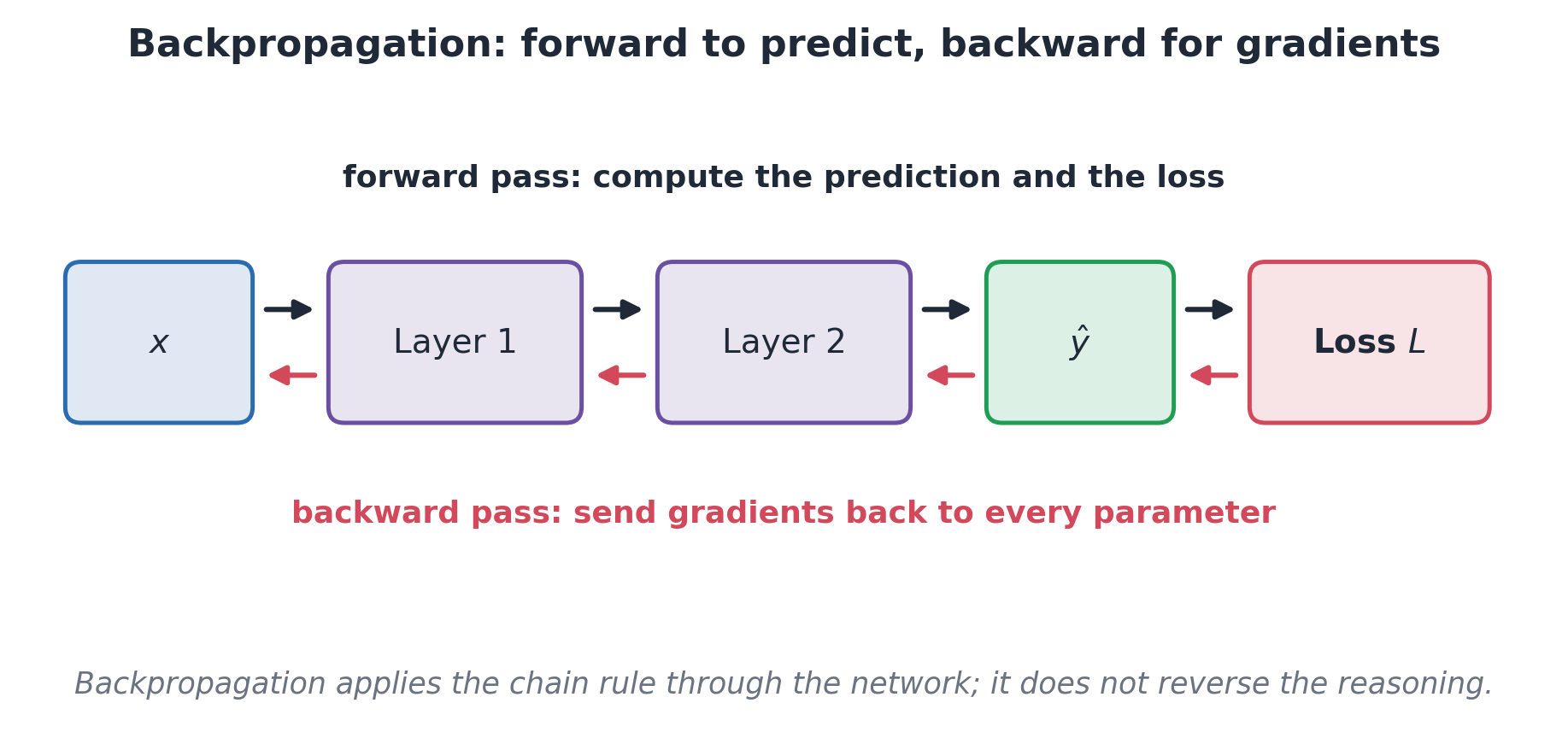
FIG. Forward Predictions and Backward Gradients

Backpropagation computes the gradients needed for training. It works backward from the loss through the network’s calculations.

The optimizer then uses those gradients to update the parameters.

Separate three actions clearly: the forward pass makes a prediction, backpropagation computes gradients, and the optimizer updates parameters. Backpropagation uses the chain rule, which relates the derivative of a sequence of functions to the derivatives of its parts. It reuses intermediate results efficiently. It does not run the prediction backward or change the parameters by itself.

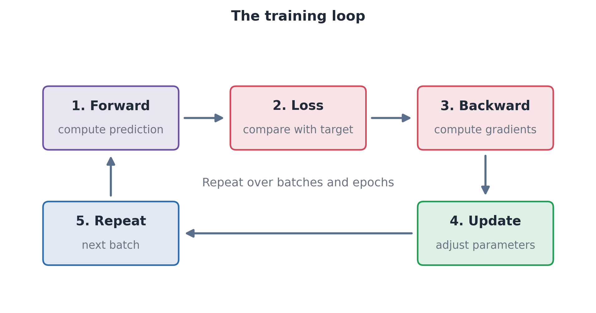
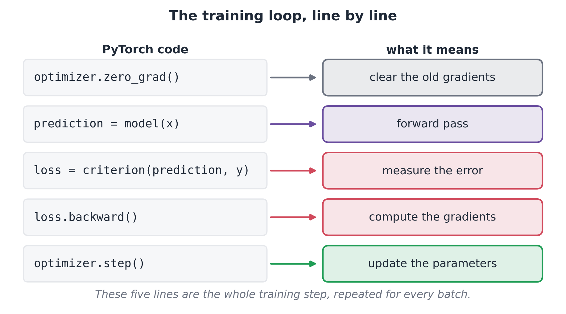
The Complete Training Loop

FIG. Prediction, Loss, Gradients, and Parameter Updates

1. Make predictions and calculate the loss.
2. Compute gradients and update the parameters.
3. Repeat with more training examples.

Each update aims to improve the model’s predictions.

Walk through the five boxes in order: forward pass, loss, backward pass, update, repeat. A single update may not lower every example’s loss, especially when using a small batch. Progress is assessed across updates and checked on validation data. This is the standard gradient-based training process used in the neural examples here.

Batches, Learning Rate, and Optimizer

A batch is a group of examples used for one update. An epoch is one pass through the training set.

With 1,000 examples and batches of 100, one epoch has 10 updates.

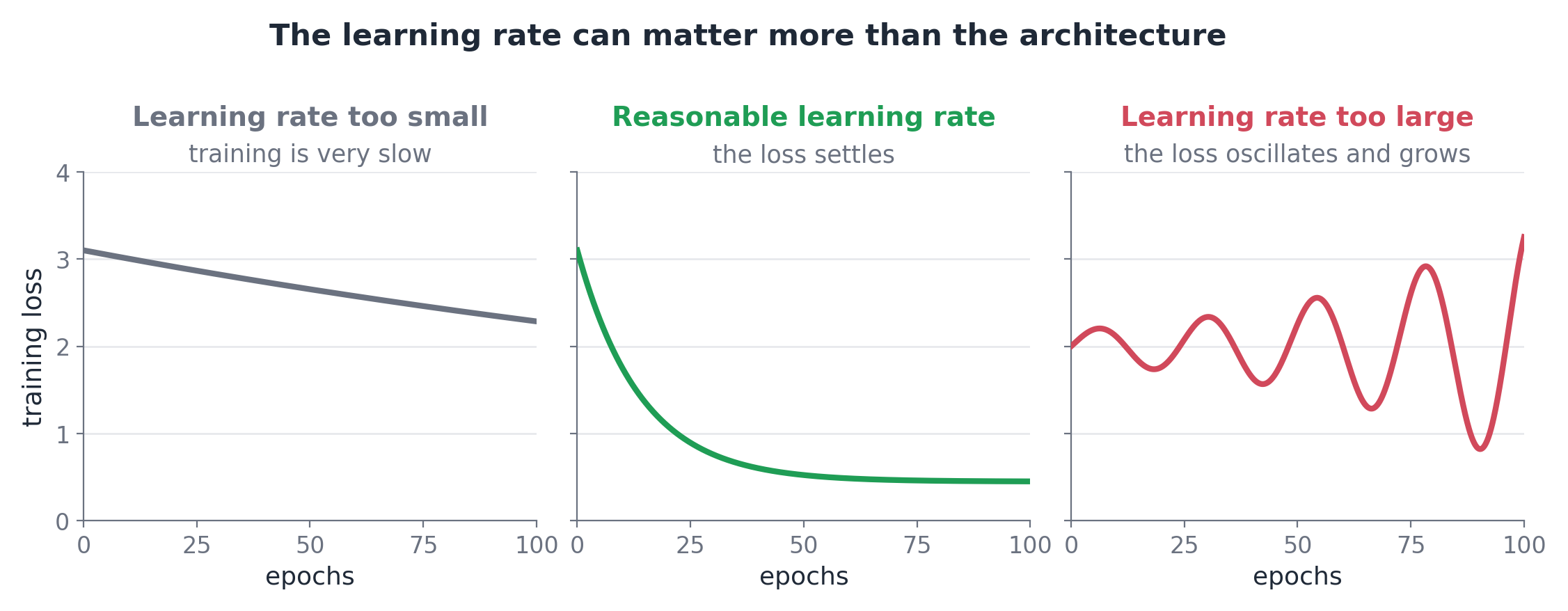
FIG. How Learning Rate Affects Training Loss

The optimizer (for example, SGD or Adam) determines the update. The learning rate sets its size: too small can be slow; too large can be unstable.

An iteration here means one parameter update. Smaller batches use less memory per update and give noisier gradient estimates. SGD uses the gradient and a learning rate; momentum also uses a running history of updates. Adam adapts updates using running statistics of gradients, while AdamW separates weight decay from that adaptation. Define weight decay later as discouraging large weights. No optimizer is best for every dataset.

Training, Validation, and Test

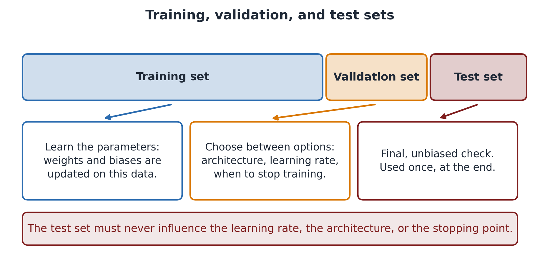
FIG. Roles of Training, Validation, and Test Data

• Training data: used to adjust the model’s parameters.
• Validation data: used to choose settings and decide when to stop.
• Test data: kept separate for the final assessment.

Do not use test results to tune the model.

Explain the roles rather than recommending a fixed percentage split. The validation set can guide architecture, learning rate, and early stopping. The test set estimates performance on the intended unseen-data setting after those choices are made. Independence, leakage prevention, and a representative split matter; merely calling a set test data does not guarantee an unbiased estimate.

Overfitting in Neural Networks

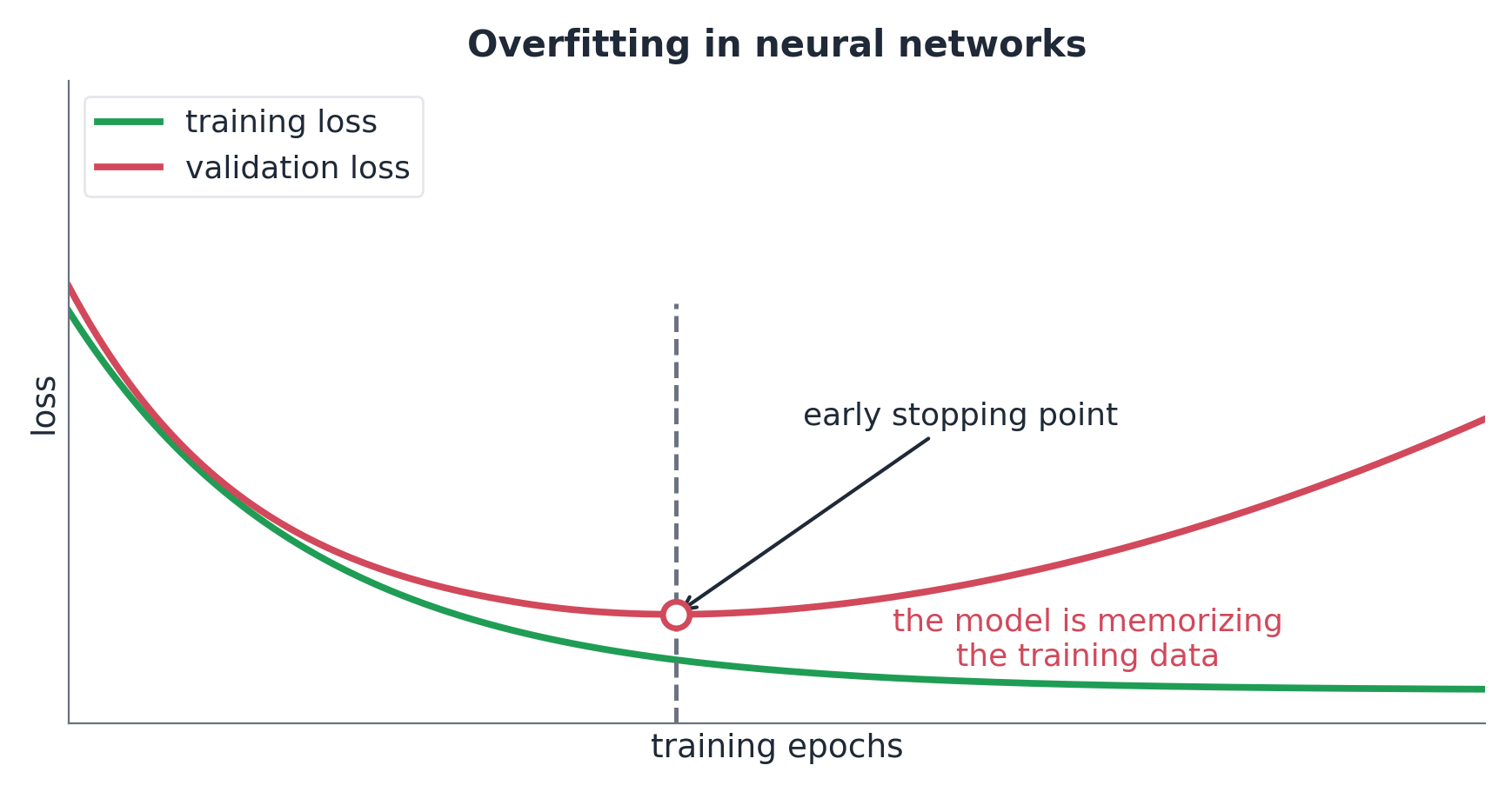
FIG. Training and Validation Loss During Overfitting

Overfitting occurs when a model fits the training examples but performs poorly on new examples.

If training loss falls while validation loss rises, consider more representative data, a simpler model, or regularization. Early stopping keeps a model from an earlier, better validation result.

Read both curves. A widening training-validation gap is a warning, although the split and measurement noise also matter. Regularization means training choices that discourage fitting accidental details. Weight decay discourages large weights; dropout randomly removes some activations during training; early stopping uses validation results to choose a stopping point. Limited labels can increase the risk, but unlabeled pretraining is not a guaranteed solution.

PyTorch

Connecting the training concepts to code.

The purpose of this section is to recognize how the concepts appear in a common framework. Students do not need to install software or implement a full project to follow these examples.

What Is PyTorch?

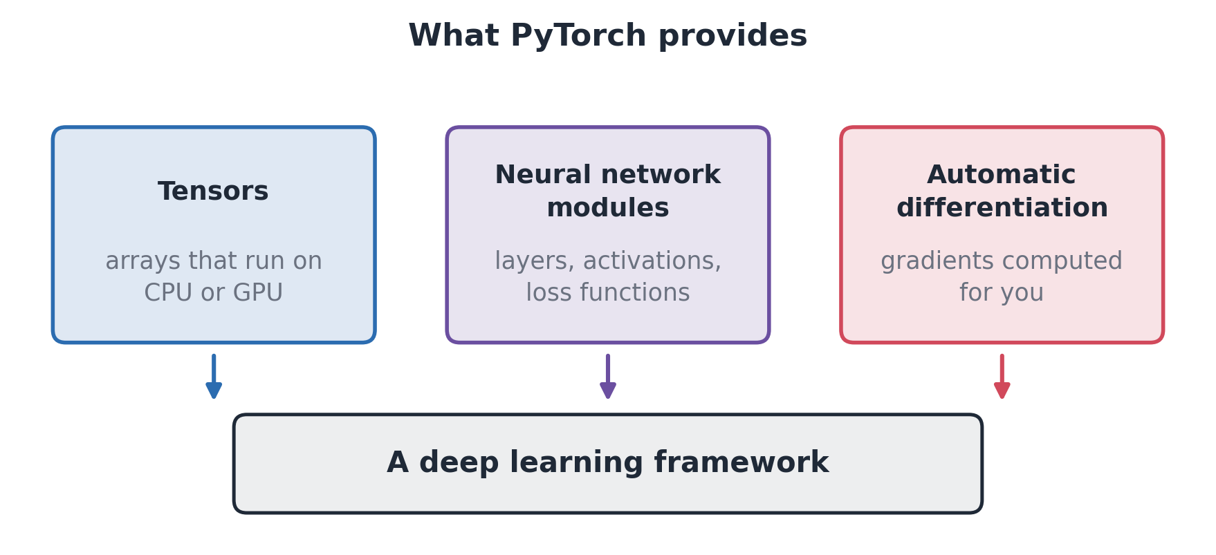
PyTorch is a Python library for building and training neural networks.

FIG. PyTorch Framework Logo

• Tensors store numerical data.
• Modules define network layers.
• Autograd computes gradients.

FIG. Tensors, Modules, and Automatic Differentiation

PyTorch provides the data, model, and gradient tools needed to implement the training loop.

Connect the three names to ideas already introduced. A tensor stores a batch of measurements. A module can represent a layer or a complete network. Autograd records the operations needed to compute gradients. PyTorch also provides optimizers and support for running calculations on supported GPUs. These are tools for implementing a model, not a guarantee that the model is appropriate.

Tensors

A tensor is an array of numbers. This separate example stores two samples with three features each.

import torch

x = torch.tensor([[0.5, 1.2, 3.1],
                  [0.7, 0.9, 2.8]])

print(x.shape)   # torch.Size([2, 3])

TABLE. NumPy Arrays and PyTorch Tensors

Capability	NumPy array	PyTorch tensor
Store numerical data	Yes	Yes
Run on a supported GPU	No	Yes
Track operations for gradients	No	Yes, when enabled

Here, rows are samples and columns are features. The feature count must match the model input.

Read the shape as rows and columns: two samples, three features per sample. This is a small standalone tensor example; the next slide uses a different example with eight input features. The tensor shown is created on the CPU. PyTorch can move compatible tensors to a supported GPU. Gradient tracking is optional; simply creating a tensor does not mean its input values require gradients.

A Neural Network in PyTorch

This example takes eight measurements and predicts one numerical value.

from torch import nn

model = nn.Sequential(
    nn.Linear(8, 64), nn.ReLU(),
    nn.Linear(64, 32), nn.ReLU(),
    nn.Linear(32, 1),
)

Linear combines inputs using weights and biases. ReLU adds a nonlinear response.

FIG. PyTorch Code and Its Network Layers

Read Sequential from top to bottom. Linear(8,64) maps eight features to 64 hidden units, and Linear(64,32) maps those to 32 units. ReLU follows each hidden linear layer. The final Linear(32,1) returns one numerical prediction without constraining it to a probability range. This is the same illustrative architecture introduced earlier; its sizes are choices to validate, not universal defaults.

The PyTorch Training Loop

For the eight-input model, x holds a batch of inputs and y its targets. With a loss function (criterion) and optimizer prepared:

optimizer.zero_grad()               # clear old gradients
prediction = model(x)               # forward pass
loss = criterion(prediction, y)     # measure the error
loss.backward()                     # compute gradients
optimizer.step()                    # update parameters

backward() computes gradients. step() changes the parameters.

FIG. Training Code and the Operation Performed by Each Line

Here x is a batch with the input shape expected by the model, and y contains its targets. The loss function compares predictions with targets; the optimizer updates the parameters. PyTorch normally accumulates gradients, so clear old gradients before computing the gradients for this update. Clearing can occur before or after the forward pass, provided it is before backward and does not discard gradients deliberately accumulated across batches. The five lines illustrate a single update, not a complete standalone training program.

Autograd and CPU/GPU Computation

Autograd records calculations and computes gradients during the backward pass. It handles the differentiation needed to train the network.

FIG. A Computation Graph Used for Automatic Differentiation

Training can run on a CPU or a supported GPU. The model and its input tensors must be on the same device.

device = "cuda" if torch.cuda.is_available() else "cpu"
model.to(device)

Gradient tracking must be enabled, and the relevant tensors must require gradients. Neural-network parameters normally require gradients; input tensors require them only when derivatives with respect to the inputs are needed. Explain that the code moves the model, and x and y must also be moved before GPU training. A GPU can speed up suitable workloads, but it is not necessary to understand or use the models in this lecture.

BREAK

FIG. From a Network to Questions About Its Use

After the break: how should we change our modeling approach when labels are scarce or data are spread across sites?

Pause and agree on a restart time. Ask students to keep one engineering example in mind for the second half. The next section changes the questions we ask about a model, not the basic meaning of prediction and training.

Part IV. Modern Modeling Paradigms for Engineering AI

Choosing an approach that fits the engineering problem.

Explain that IV.A–D cover different modeling choices. These topics can sometimes be combined. They are not levels of sophistication or a sequence of required methods.

IV) Beyond One Dataset and One Model

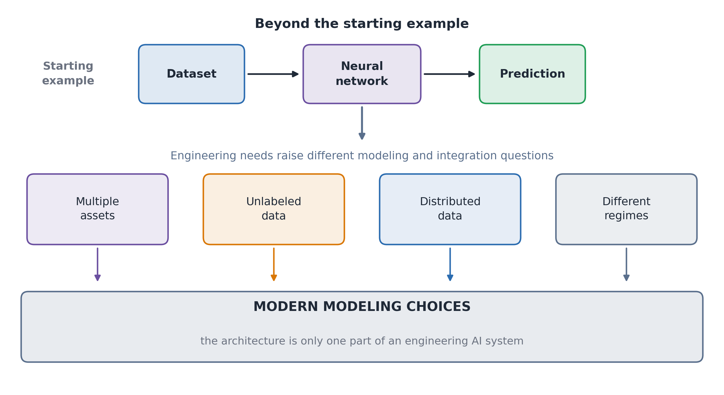
So far, we have used one dataset to train one predictor. Other situations raise new questions:

FIG. Learning Situations Beyond One Dataset and One Model

Choose the approach from the problem: available labels, related machines, and data-sharing limits. The next sections address these different needs.

Use the figure as a set of questions. Multiple assets means related machines or systems. Unlabeled data have measurements but no externally supplied target for the task. Distributed data are held at different sites. Operating regimes are different conditions, such as a ship cruising or maneuvering. None of these automatically requires a particular method.

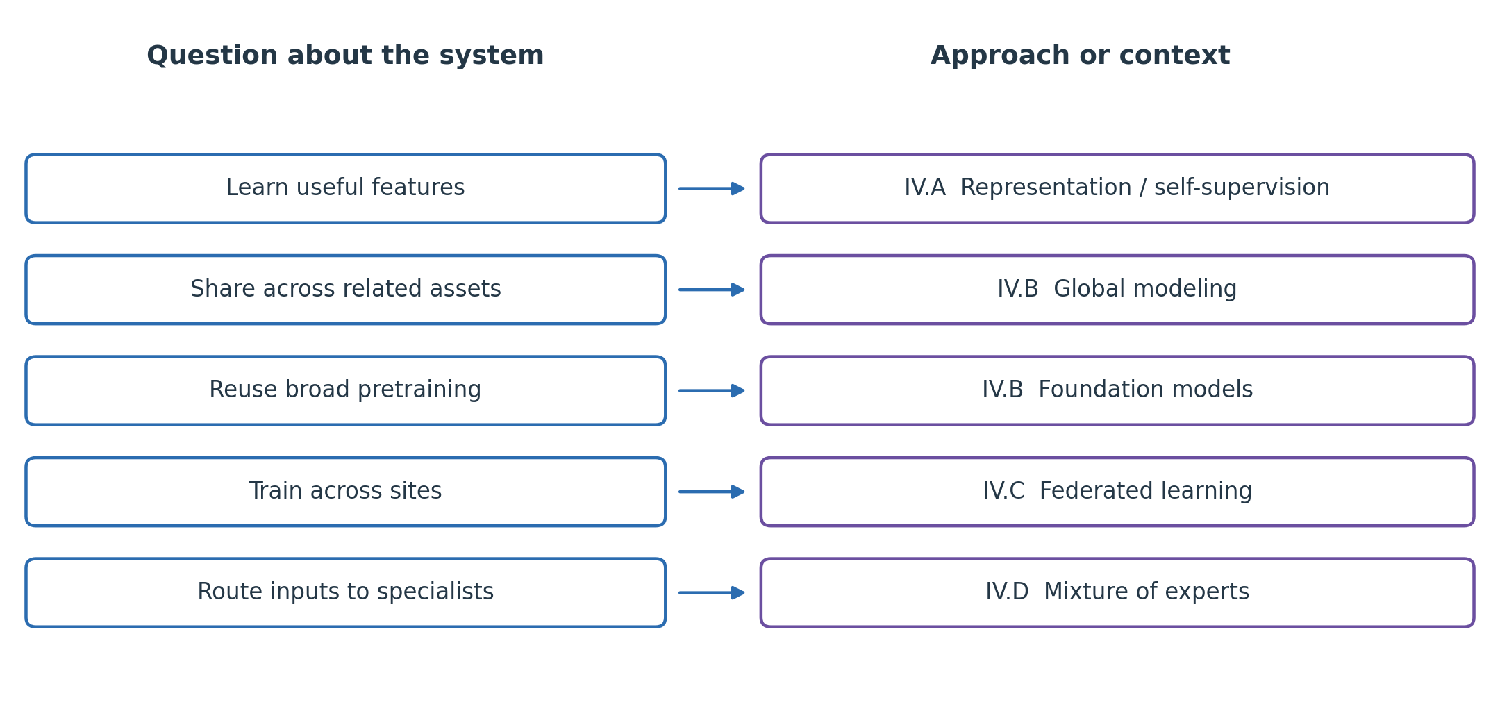
IV) A Map of Modeling Approaches

FIG. Different Questions About an AI System

These are different dimensions of a system. They can overlap and be combined.

Read the map as questions, not ranks. Autoencoders are one representation-learning method. A system can use a global predictor trained through federation. The map separates model purpose, training organization, and architecture.

IV.A) Representation Learning

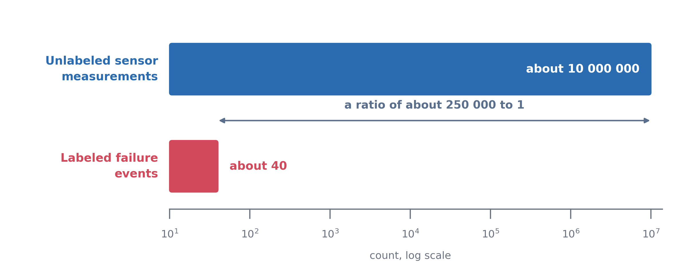
A label is a known target, such as a confirmed machine fault. Factories may collect years of sensor readings but record only a few confirmed faults.

FIG. Many Sensor Recordings but Few Confirmed Failures

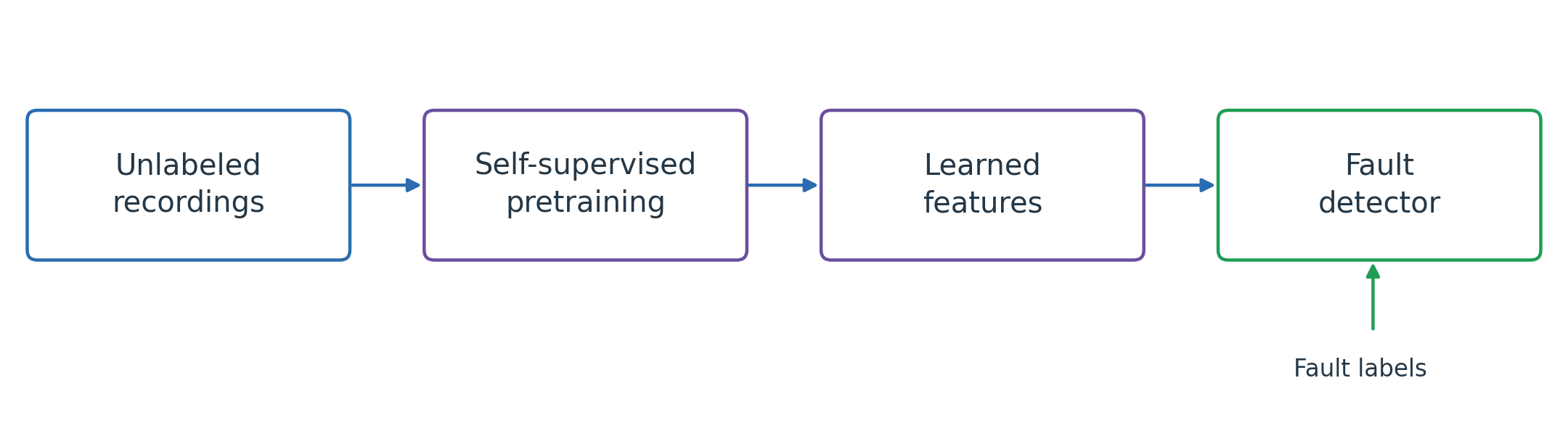
Representation learning learns useful features from data. Here, the aim is to learn from many unlabeled readings, then use the few fault labels to train a detector.

Use the example of ten years of vibration data and forty documented bearing failures. A label is not merely the name of a column; it is the known outcome for a training task. Representation learning can be supervised or use unlabeled data. Here the interest is in learning from the many measurements before fitting a fault detector with scarce labels. The learned features still need evaluation on that final task.

IV.A) From Measurements to Useful Features

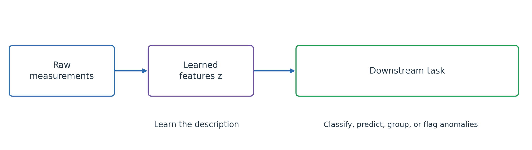
Representation learning learns features that help describe the input 1.

FIG. From Measurements to Features and Downstream Tasks

A downstream task uses those features for a later purpose, such as fault detection.

Autoencoders are one method. Representation learning can also use supervised or self-supervised training.

Ask what a useful vibration feature should preserve: a pattern associated with faults, rather than only background noise. The downstream task determines whether the representation helps. Classification predicts a category, regression a number, clustering groups examples, anomaly detection flags unusual examples, and forecasting predicts future values. These are possible uses, not guarantees.

IV.A) Representation and Autoencoders

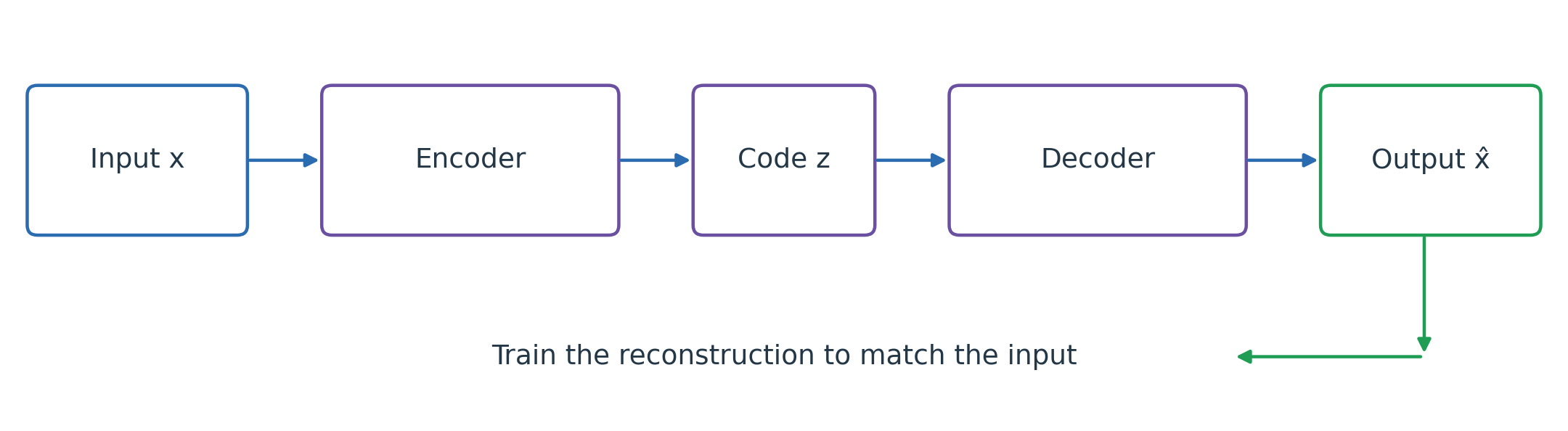
An autoencoder learns to reconstruct its input: \hat{x}\approx x.

FIG. Encoder, Latent Code, and Reconstruction

The encoder maps x to learned features z, the latent code. The decoder reconstructs \hat{x} from z.

A compact code encourages the model to preserve structure needed for reconstruction. Training minimizes \lVert x-\hat{x}\rVert^2: the sum of squared reconstruction differences. Check whether z helps the intended task.

Define latent representation as the encoder output z: variables learned by the model rather than directly measured. A bottleneck limits the space available to represent the input, but it does not guarantee physically meaningful features. An autoencoder can reconstruct background variation rather than information relevant to faults. High reconstruction error indicates an unusual sample, not necessarily a fault. The input supplies the reconstruction target, so an external target label is not needed for that stage.

IV.A) Three Autoencoder Variants

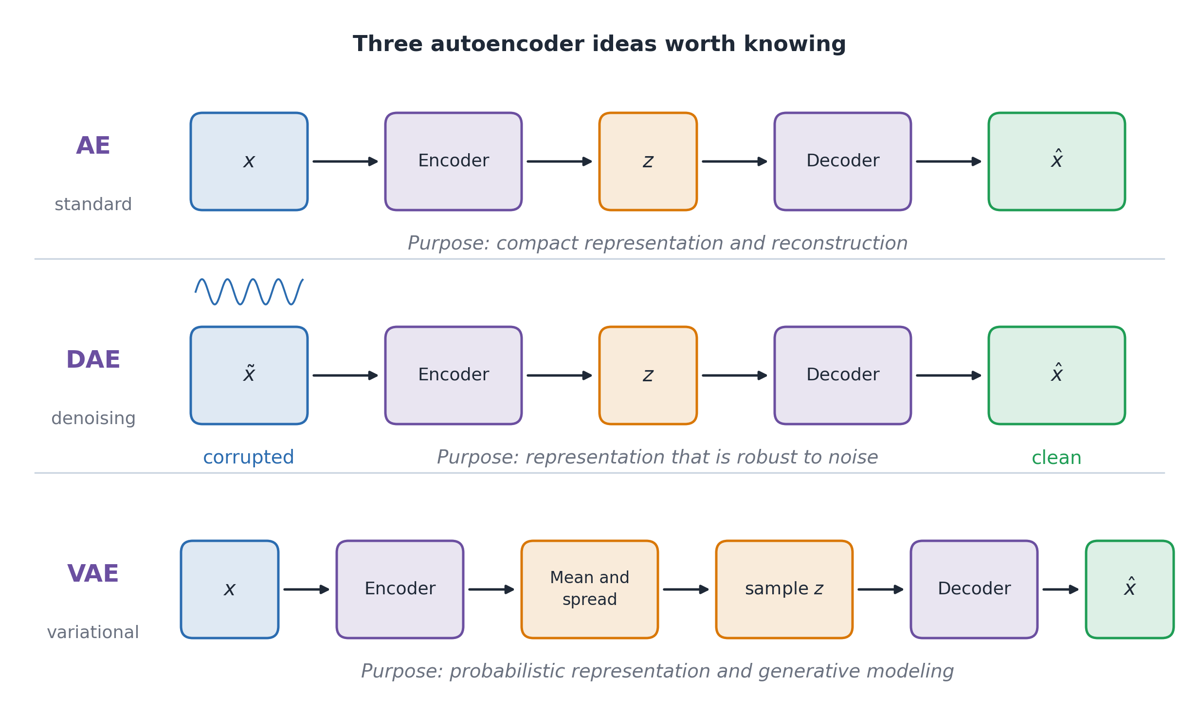
FIG. Standard, Denoising, and Variational Autoencoders

• Standard autoencoder: reconstruct the input.
• Denoising autoencoder: reconstruct a clean input from a corrupted version.
• Variational autoencoder (VAE): learn a probabilistic latent representation that supports generation.

Choose the training task to match the aim: reconstruct inputs, remove noise, or learn to generate samples.

The three diagrams show related ways to learn from inputs without external task labels. A denoising model learns to recover information after a specified corruption. A VAE learns parameters of a latent distribution and uses a regularized objective, allowing generation by sampling. Generation alone does not ensure a feasible engineering design. Self-supervised objectives also include masking and predicting parts of the input or learning which views should be similar. The task used for pretraining determines what information the representation preserves, so good reconstruction does not guarantee good fault detection.

IV.A) Self-Supervised Learning

Supervised learning: use known task labels. Self-supervised learning: construct targets from the data themselves.

• Hide a sensor reading and predict it from the others.
• Use earlier time-series observations to predict a later region.

FIG. Self-Supervised Pretraining Followed by Fault Detection

Self-supervision is broader than autoencoders. The training task should preserve information useful for the downstream task.

In the illustrated workflow, ten years of recordings support pretraining and forty labeled failure events support a later fault-detection task. Pretraining means initial training whose learned parameters are reused. Small labeled data are part of this example, not part of the definition of a downstream task. Ask students where the target comes from when a reading is hidden. The original reading supplies the answer. Forecasting can also create targets from observed sequences.

IV.B) Local and Global Models

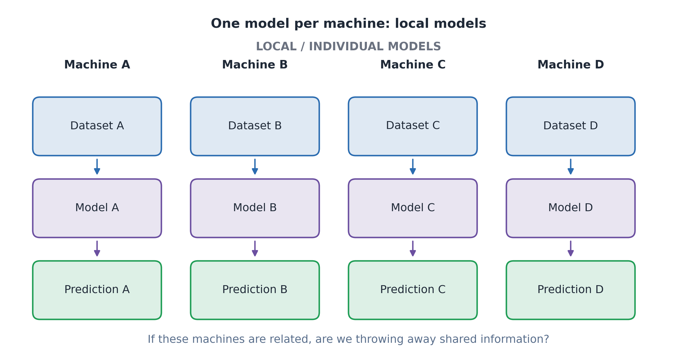
Suppose a company operates many similar pumps. Should each pump have its own prediction model?

FIG. Separate Models for Individual Machines

A local model is trained for one asset. It can capture that pump’s behavior, but may have little data. If each pump has little history, consider learning across related pumps.

An asset here is an individual machine or system. A fleet is a collection of related assets. Explain the tradeoff: a local model focuses on one pump but can use only that pump’s history. This motivates the next slide, which considers learning from several related assets together.

IV.B) Global Modeling

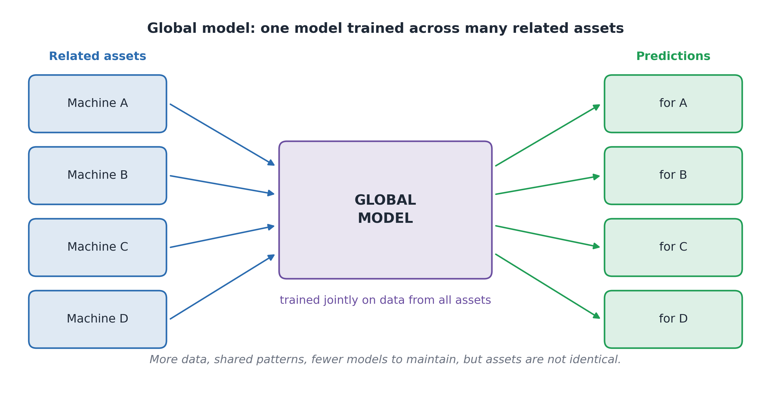
A global model learns from several related assets and makes predictions for them 3.

FIG. One Model Learns Across Several Machines

Shared data may help when each asset has little history. However, machines can differ in age, load, and environment.

Compare performance for each asset, as well as overall.

Contrast a separate model for every pump with one model trained across pumps. A global model may use asset identity or operating conditions as inputs. It can improve predictions but may also fit some assets poorly. Compare it with local models on the intended deployment setting. Global describes the scope of a model, while federated describes how training is organized; this illustration uses centrally pooled data.

IV.B) Global and Foundation Models

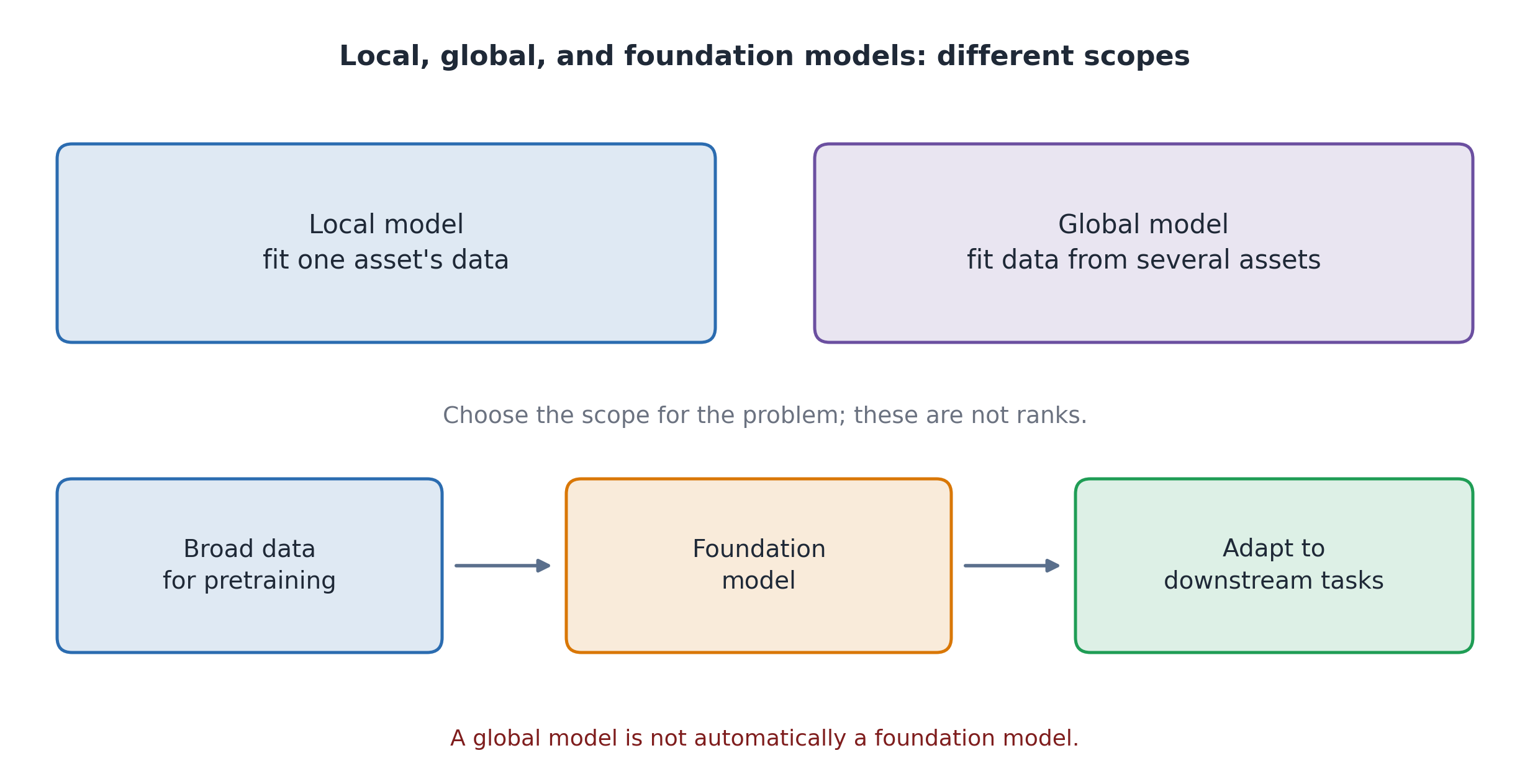
A global model shares learning across related assets. A foundation model is trained broadly so it can be adapted to many tasks 4.

FIG. Global Modeling and Foundation-Model Pretraining

Pretraining is the initial learning stage. Adaptation, such as fine-tuning, prepares the model for a particular task.

Global modeling shares learning across assets; foundation models support reuse across tasks.

Give an example: a global model predicts remaining life across a fleet, while a foundation model might be adapted to forecasting, classification, and other tasks. Pretraining may use supervised or self-supervised objectives. Foundation models are characterized here by broad training and downstream adaptability, not size alone. The diagram compares different choices; it is not a required progression from local to global to foundation modeling.

IV.B) Global vs Foundation: What Is Shared?

TABLE. Global Models and Foundation Models

Question	Global model	Foundation model
Main purpose	Share learning across related assets	Reuse broad pretraining across tasks
Example data	Histories from many pumps	Broad, diverse sensor recordings
Example use	One fault-prediction task across pumps	Adapt to forecasting or fault diagnosis
Further training	May be trained for the shared task	Fine-tuning updates pretrained parameters

More data alone do not turn a global model into a foundation model.

Pretraining builds reusable knowledge; adaptation applies it to a target task. Fine-tuning is one form of adaptation.

Read each row across. Local/global describes the scope across datasets or assets. Foundation describes broad pretraining and adaptability. These properties are not mutually exclusive: a foundation model can be adapted for a task across many pumps. In this comparison the global model serves one task, which is an example rather than a universal restriction. Reusing a model still requires evidence on the new task.

IV.B) Foundation Models for Engineering

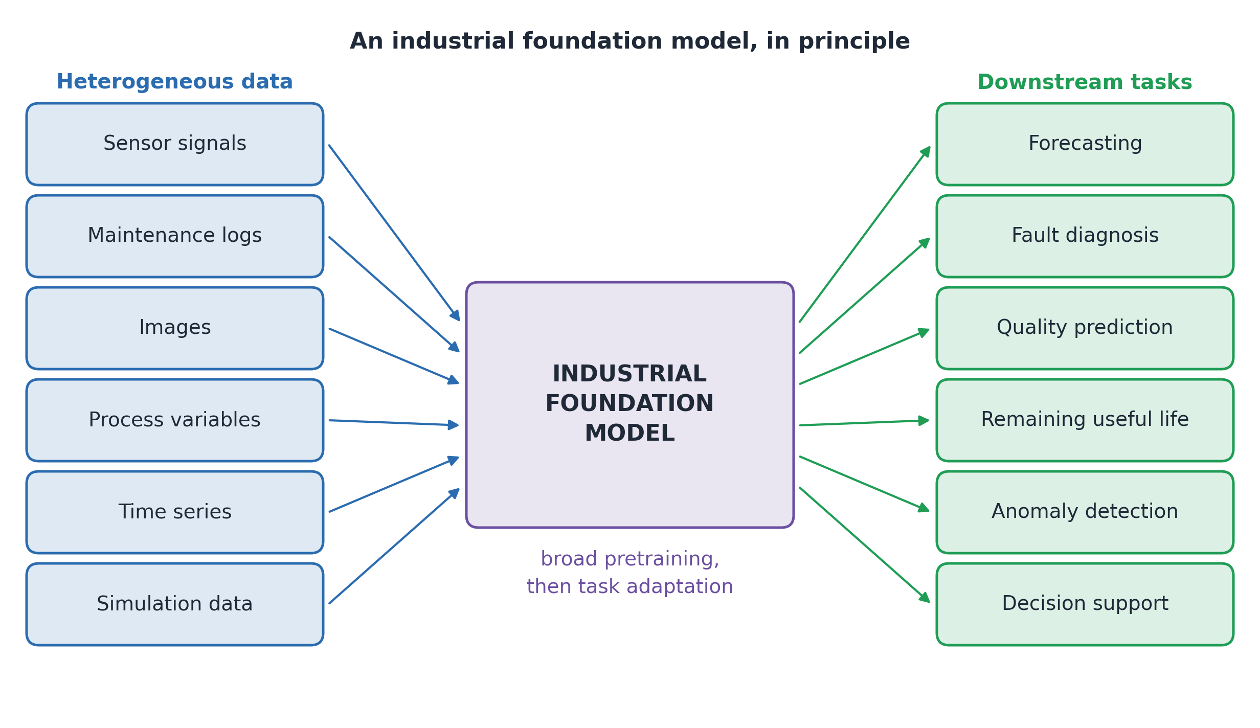
A model pretrained on broad engineering data could be adapted to tasks such as fault detection or forecasting.

FIG. Foundation Models for Engineering Tasks

Before using it, check whether its training data resemble your application: sensors, units, equipment, and operating conditions may differ.

Compare the adapted model with established methods on your own task.

Explain that a foundation model is not necessarily a language model or a chatbot. Engineering data can include sensor sequences, images, process records, and simulations. Reuse is attractive when task-specific labels are limited, but proprietary data and differences between sites create difficulties. Broad pretraining does not establish accuracy or reliability in a new operating environment.

IV.C) Federated Learning

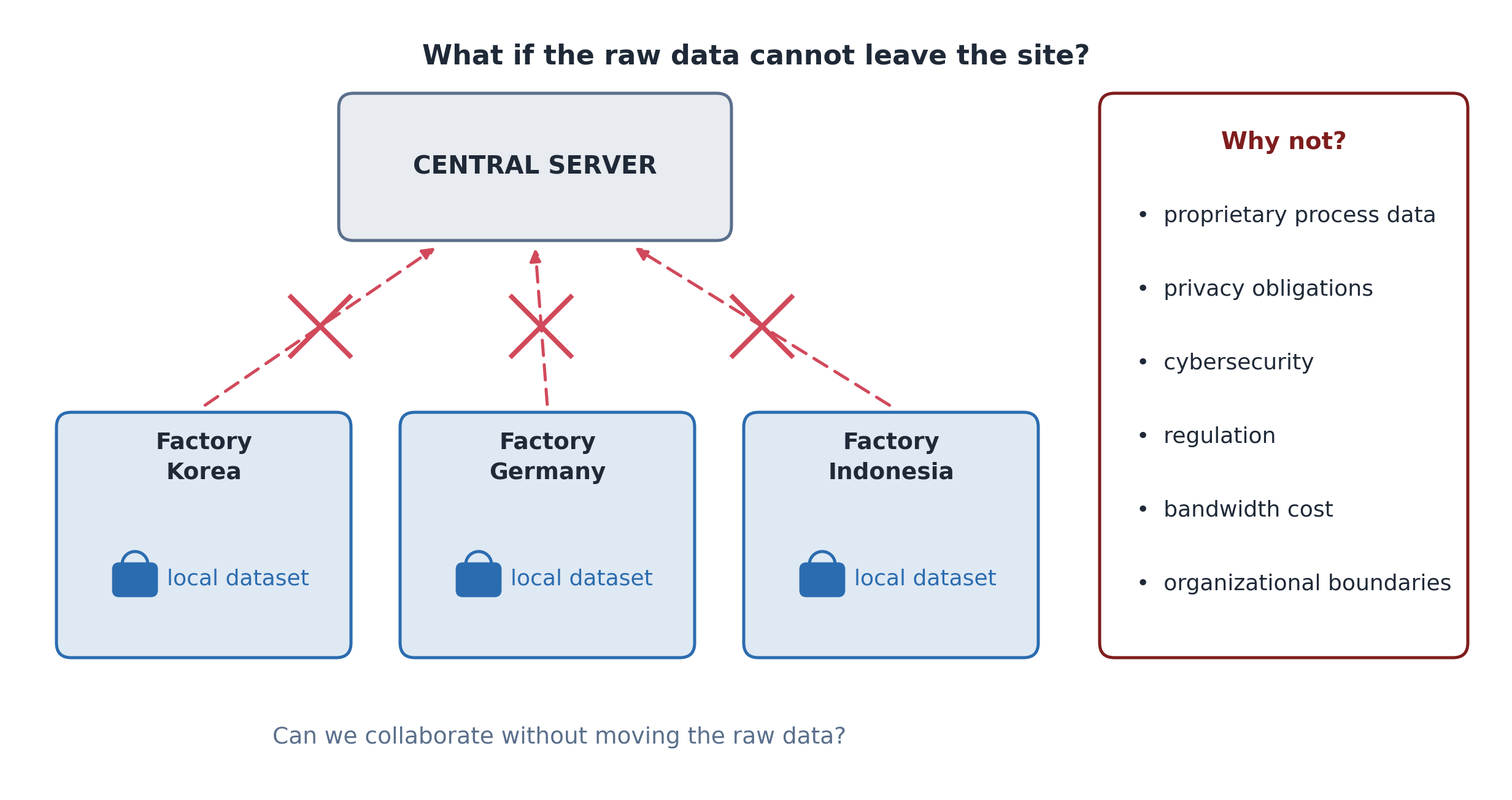
Several factories have useful data but cannot pool their raw records. Can they learn together?

Federated learning trains a shared model across sites without collecting their raw training data in one place.

FIG. Factories Hold Their Training Data Locally

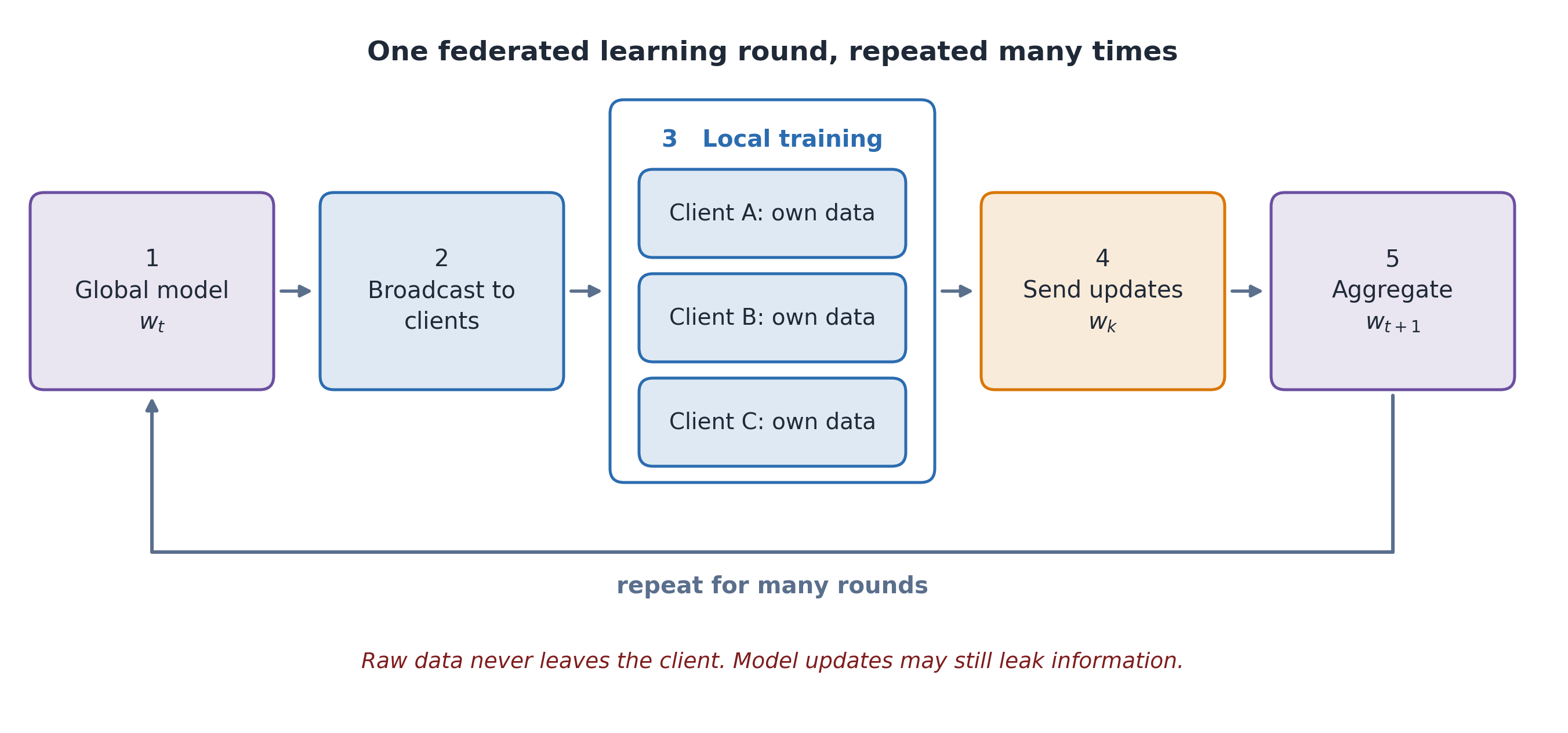
Each participating factory is a client. It trains locally and shares model updates.

A participating site is called a client. Model updates contain learned parameter information, not the original measurement records. The illustration uses factories in three countries, but the same idea applies to other organizations or devices. Keeping data local does not by itself guarantee privacy. Start by checking that the participants have a useful shared learning problem.

IV.C) One Federated Training Round

FIG. One Round of Federated Learning

1. Send the shared model; each client trains on local data.
2. Combine what clients learned: the server merges their updates into the next shared model.
3. Repeat with the next participating clients.

Trace the arrows before discussing arithmetic. Clients begin from the same shared parameters and train copies using their local datasets. The server combines corresponding parameters. FedAvg is the sample-count-weighted averaging method introduced next; other aggregation methods also exist.

IV.C) FedAvg: A Weighted Average

FedAvg weights client parameters by local example counts 5.

TABLE. Client Example Counts and FedAvg Weights

Client	Training examples	Share of total
A	1,000	50%
B	500	25%
C	500	25%
Total	2,000	100%

w_{\mathrm{global}}=0.50w_A+0.25w_B+0.25w_C=\sum_k\frac{n_k}{N}w_k

w_k: client k’s parameters after local training; n_k: its example count; N: total examples across participating clients.

A contributes half because it has half the examples. Average corresponding parameters.

Compute 1000/2000, then 500/2000. If one corresponding parameter is 2 at A, 4 at B, and 6 at C, its new value is 0.5×2 + 0.25×4 + 0.25×6 = 3.5. This averages parameters, not final predictions. All participating clients use the same parameter structure and start from the shared model. Sample-count weighting does not guarantee equal performance at every site.

IV.C) Centralized vs. Federated Learning

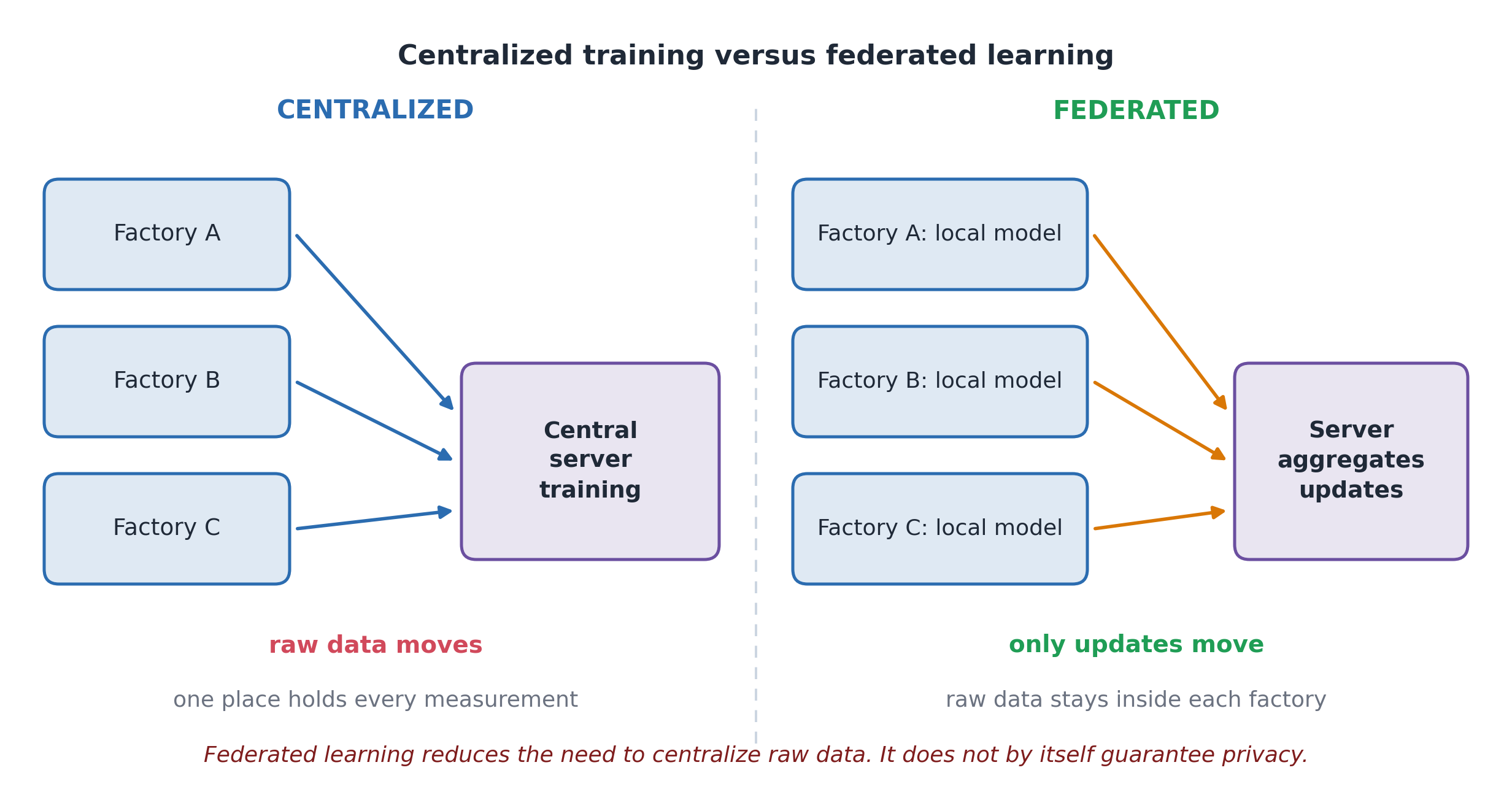
FIG. Centralized Data and Federated Model Updates

• Centralized training: data move to the training system.
• Federated training: local model updates move between sites and the server.

Keeping raw data local does not guarantee privacy. Updates can reveal information, so extra protection may be needed.

Point to what travels along each arrow. Secure aggregation can limit what the server sees about individual updates, and differential privacy can reduce information leakage by adding calibrated randomness. These measures have costs and do not replace broader security practices. Keep the main distinction visible: where training data remain and what is communicated.

IV.C) Federated Learning: Different Data

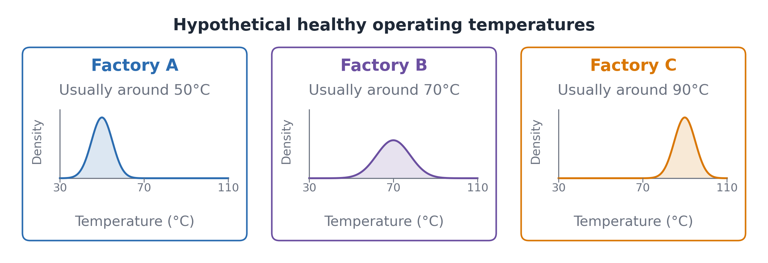
Factories train one shared model, but healthy operating temperatures differ.

FIG. Different Normal Temperatures Across Factories

The risk: a detector could mistake Factory C’s healthy 90°C readings for a fault.

IID means independent and identically distributed. These factories have different distributions, so their data are non-IID.

So, good overall accuracy is not enough. Check the shared model at every factory before using it.

Define a client as one participating factory. The temperatures are hypothetical healthy values, not operating limits. A fault detector that treats high temperature as abnormal without considering the machine’s conditions could falsely flag healthy operation at another site. The curves are distributions of measurements, not time histories. IID means independent and identically distributed samples; the figure illustrates failure of the identical-distribution assumption. Dependence between nearby time-series readings is another issue. Non-IID data can complicate training, but they do not make federated learning impossible.

Close with the practical decision: overall accuracy can hide poor performance at one site. Before using the shared detector, check missed faults and false alarms separately at each factory.

IV.D) Mixture of Experts: Specialization

A ship uses fuel differently when maneuvering, cruising, or operating in heavy weather. These are different operating regimes.

FIG. Different Operating Regimes Motivate Expert Models

If one predictor consistently struggles in some regimes, consider several specialized predictors. First compare with a model that includes the operating conditions as inputs.

This is a model-design choice rather than a required solution to the preceding federated-learning problem. Plot prediction errors against operating conditions before introducing complexity. The diagram labels experts A, B, and C without claiming that they have learned human-named regimes. Gate weights are illustrative; any interpretation of an expert’s role must be checked.

IV.D) Mixture of Experts

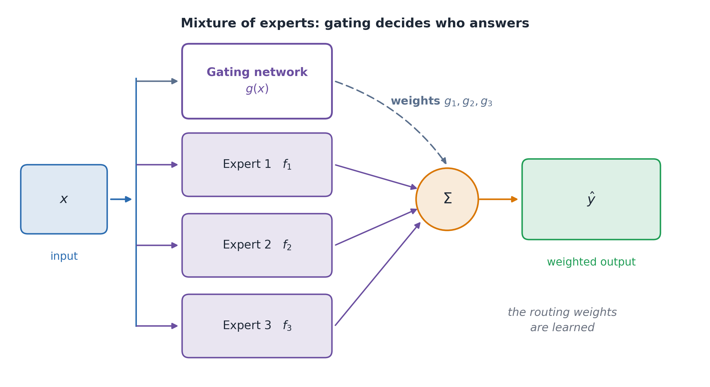
A mixture of experts combines several submodels. A gating network learns to assign their contributions from the input. The gate and experts train together 6.

FIG. Input-Dependent Contributions from Expert Models

f_i(x) is expert i’s prediction. g_i(x) is the weight given to that expert for input x.

The model can rely on different experts for different operating conditions.

For this mixture, the gate supplies nonnegative weights that sum to one. Experts and gate are trained together. A different input can receive a different mixture of predictions. An expert need not correspond to a physical regime unless that was designed or verified. This is a form of combining models; the learned, input-dependent gate is the central idea.

IV.D) A Gate Chooses the Expert Contributions

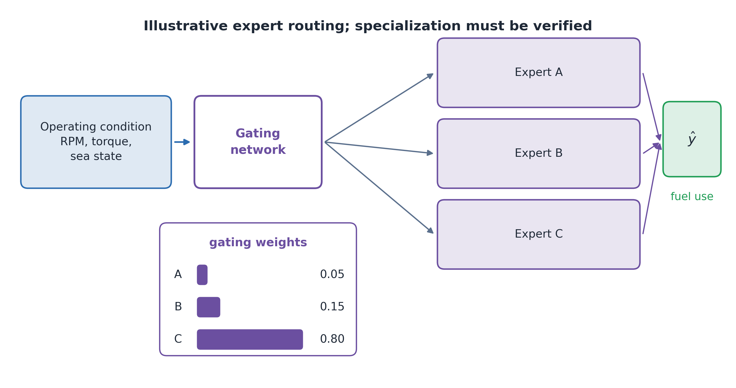
Example input: 18 knots, 0.5 m waves, 75% engine load. The gate selects these illustrative weights:

TABLE. Gate Weights and Expert Fuel Predictions

Expert	Gate weight	Predicted fuel use
1	0.80	20 tonnes/day
2	0.05	30 tonnes/day
3	0.15	24 tonnes/day

\hat y=0.80(20)+0.05(30)+0.15(24)=21.1\text{ tonnes/day}

In general, \hat y=\sum_i g_i(x)f_i(x): f_i(x) is expert i’s prediction; g_i(x) is the gate’s weight for input x.

Expert 1 has the most influence here (80%). The weights are nonnegative, sum to one, and can change with the input.

The weights sum to one. Calculate each contribution, then sum them. These are hypothetical model outputs, not measured ship data. The gate responds to the input; it does not simply choose whichever prediction is closest to an unknown target. Expert numbers do not establish physical roles such as cruising. Such roles require analysis. All experts run in this small example; the next comparison introduces sparse routing.

IV.D) Experts and Conventional Ensembles

Both approaches combine predictions from several models. Their main difference is how the contributions are chosen.

TABLE. Conventional Ensembles and Mixtures of Experts

	Averaging/voting ensemble	Mixture of experts
Combine predictions	Average or vote	Use a learned gate
Depend on the input?	Usually the same combination rule	Gate weights depend on the input
Which models run?	Usually all members	All, or a selected subset

A sparse mixture uses only a few experts for each input, reducing computation.

Check whether input-dependent specialization improves predictions enough to justify the extra complexity. Also check that the gate uses its experts effectively.

Mixtures of experts can also be called ensembles; the table compares them with conventional averaging or voting. Sparse routing trades the cost of evaluating every expert for the cost of choosing a subset. Training may become unbalanced if one expert receives most examples. Compare accuracy, computation, and stability with a simpler model, and verify any physical interpretation assigned to experts.

IV.E) Look Beyond the Network Diagram

A network diagram alone does not tell us how a model is used. Ask:

• Task: what does the model need to predict or represent?
• Training: what objective does it learn from?
• Data: which examples and sites contribute?
• Use: how will the result support an engineering decision?

The same type of network can play different roles, depending on these choices.

For example, an MLP can predict strength, form part of an autoencoder, be trained across federated clients, or serve as an expert. Some choices change the architecture, while others change training or deployment. Do not infer an entire modeling approach just from the presence of an MLP.

IV.E) Scope of These Approaches

The lecture covered four groups of modeling choices:

• IV.A: learn useful features, including from unlabeled data.
• IV.B: share learning across assets or adapt pretrained models.
• IV.C: train across sites while keeping raw data local.
• IV.D: combine specialized predictors.

Choose approaches for the needs they address; combine them when useful. These groups are not a complete list of AI methods.

Use this slide to help students organize what they have seen. The labels are navigation aids, not levels of maturity. Other relevant subjects include multi-task, continual, graph, reinforcement, and multimodal learning; they are not covered in detail here. Transfer and adaptation were introduced only as needed to explain foundation models.

IV.E) Choosing an Approach

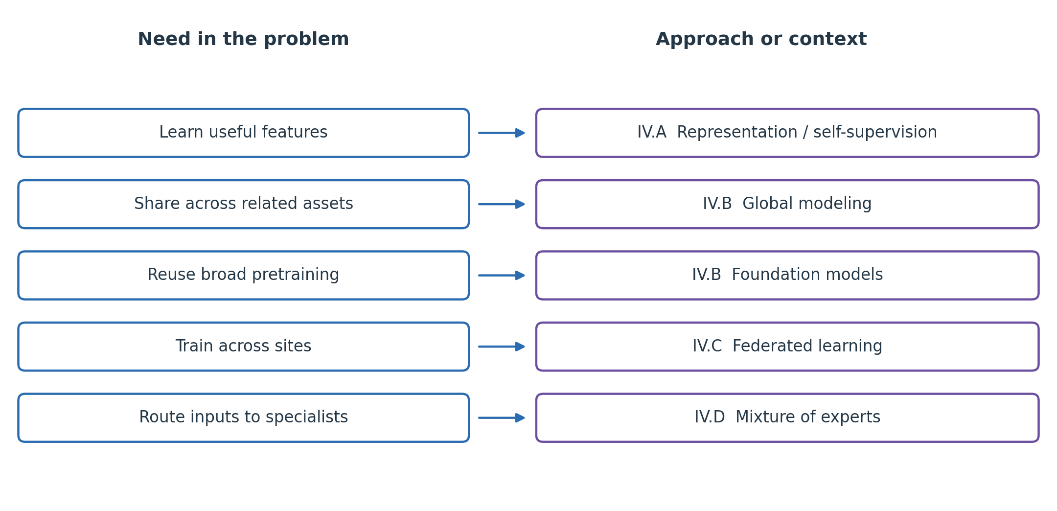
FIG. Problem Questions Suggest Candidate Approaches

This is a guide, not an exclusive decision tree. Several approaches may be combined; compare choices with a suitable baseline.

The arrows suggest candidates, not unique answers. Scarce labels may motivate self-supervision; many related assets may motivate a global model; restricted data movement may motivate federation if a shared model is useful. Distinct regimes may justify experts only after evaluating a simpler model. Several choices may be combined, but none is automatically necessary.

IV.E) Comparing the Approaches

TABLE. Learning, Sharing, and Combining Models

Approach or context	When to consider it	Main idea	What to check
Self-supervised features	Few task labels	Learn from targets created from the inputs	Do the features help the final task?
Global model	Many related assets	Share learning across assets	Performance on each asset
Foundation model	Several tasks to adapt to	Reuse a broadly pretrained model	Fit to the new data and task
Federated learning	Data stay at different sites	Train locally and combine updates	Local performance, privacy, communication
Mixture of experts	Different operating conditions	Learn how to combine specialized models	Accuracy, cost, use of each expert

Ask what is learned, shared, or reused. These choices describe different parts of a learning system.

Give students time to compare the five rows: learning features, sharing a model across assets, adapting a pretrained model, organizing training across sites, and routing inputs to specialists. A foundation model is defined by broad pretraining and adaptability. Do not rank the rows by sophistication; ask which rows could describe the same system, and which checks would matter most for one example discussed in class.

IV.E) Which Approach Would You Choose?

For each situation, suggest an approach and explain why it may help. More than one answer may be reasonable.

• A. Ten years of vibration data, but only 40 confirmed bearing failures.
• B. Five companies with similar machines cannot share raw production data.
• C. A ship’s fuel use differs during maneuvering, cruising, and heavy weather.

Give pairs time to discuss a choice and one validation check. A may suggest self-supervised features followed by a supervised fault detector. B may suggest federated learning, provided sharing a model is useful and privacy risks are addressed. C may suggest experts, but first compare with one model using operating-condition inputs. Reward justified baseline choices and acknowledge uncertainty; the exercise is not a matching test with one mandatory answer.

IV.E) Read the Method, Not Just Its Name

A paper describes its model as an industrial foundation model. Before accepting that description, ask:

• What are the inputs and outputs?
• What data were used for pretraining, and how broad are they?
• What loss or objective is used for training?
• How much adaptation does each new task require?
• Does the method improve on a suitable baseline on unseen cases?

Judge the method by what it does and how it is evaluated.

Use the foundation-model title as a concrete paper-reading exercise. Identify the architecture, objective, pretraining data, and adaptation procedure, then inspect the evaluation. A method can be useful even if its title uses terminology loosely. The same reading habits apply to papers about federated learning, global models, and mixtures of experts. Students should leave with questions they can use to assess a paper, not only a list of model names.