Lecture 4: Time Series Forecasting and Anomaly Detection

Predict expected behavior, recognize meaningful deviations

Special Topics in Artificial Intelligence (STAI 2026)

Week 4: Overview What Changes When Data Has a Time Order?

Machine vibration, electricity demand, traffic, sales, and heart rate all change over time.

• Forecasting: can we predict what happens next?
• Anomaly detection: is what happened consistent with what we expected?

Figure 1. One history, two questions.

Ask which readings would help predict the next machine temperature. Recent history and operating conditions both matter. The same expected behavior can later help judge an observed reading. All numerical examples and plotted sensor data in this deck are hypothetical teaching examples, not measurements from a real machine.

Week 4: Overview Today’s Roadmap

Today’s story: first we learn to predict what comes next. Then we learn to notice when what happens is not what we expected.

Part I: Forecasting, including exercises

I.A Time-series data · I.B Forecast definition · I.C Forecasting methods · I.D Forecast evaluation · I.E Distribution shift and adaptation.

BREAK

Part II: Anomaly detection, including discussion

II.A Understanding anomalies · II.B Normal behavior · II.C Detection methods · II.D Detection evaluation · II.E Monitoring · II.F Decisions.

We will mainly use machine temperature and RPM, with other sensors where useful. Week 6 applies these ideas in a practical session. Full explanations, worked answers, and a glossary are in the lecture notes on the Week 4 page.

Use the opening questions, numerical examples, and short discussions throughout the two parts. RPM means revolutions per minute. All examples are illustrative; temperatures are not operational recommendations.

I.A) Understanding Time-Series Data Reading a Time-Series Graph

A time series is a sequence of observations recorded over time.

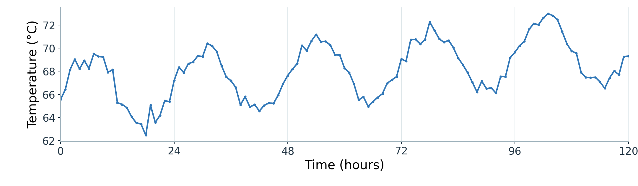
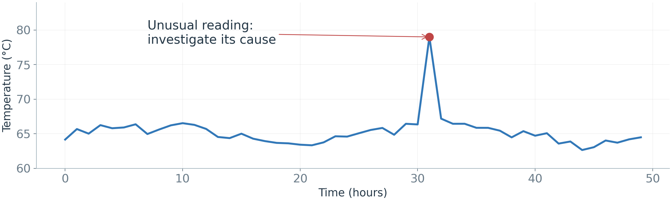
Here, each point is an hourly machine-temperature reading. Time is on the horizontal axis; temperature is on the vertical axis.

Figure 2. Hourly temperature readings from one machine, using illustrative data.

What can you see? An overall rise, repeating peaks, and smaller irregular changes. We will separate these patterns next.

Let students describe the raw line before naming the components. Every point belongs to the same machine, so its timestamp and order matter. Shuffling the readings would change the apparent pattern. The series is synthetic, generated for this lecture. The following decomposition uses exactly these same observations. These temperatures are not operational recommendations.

I.A) Understanding Time-Series Data Decomposition: Why Separate the Patterns?

Time-series decomposition separates an observed series into estimated components. For an observed value y_t at time t, an additive decomposition is:

y_t=T_t+S_t+R_t

• Trend (T_t): the underlying level and longer-term direction.
• Seasonality (S_t): variation that repeats at a regular interval, such as each day.
• Remainder (R_t): what remains after removing the estimated trend and seasonality.

Why use it? Separate long-term change from repeated variation, then examine what remains.

Here y_t is the observation at time t. The three components refer to that same time, and their sum reconstructs the observation. Trend is shorthand for the trend-cycle component in the reference. Seasonal patterns repeat at a known interval, while cycles need not have a fixed period. Real components are estimated rather than directly observed, so their values depend on the decomposition method and its settings. Additive decomposition is useful when the seasonal fluctuations have roughly constant size; it is not the only form of decomposition. Decomposition is an analysis tool and is not required by every forecasting model. No decomposition algorithm needs to be derived at this point.

I.A) Understanding Time-Series Data Decomposition: Reading the Components

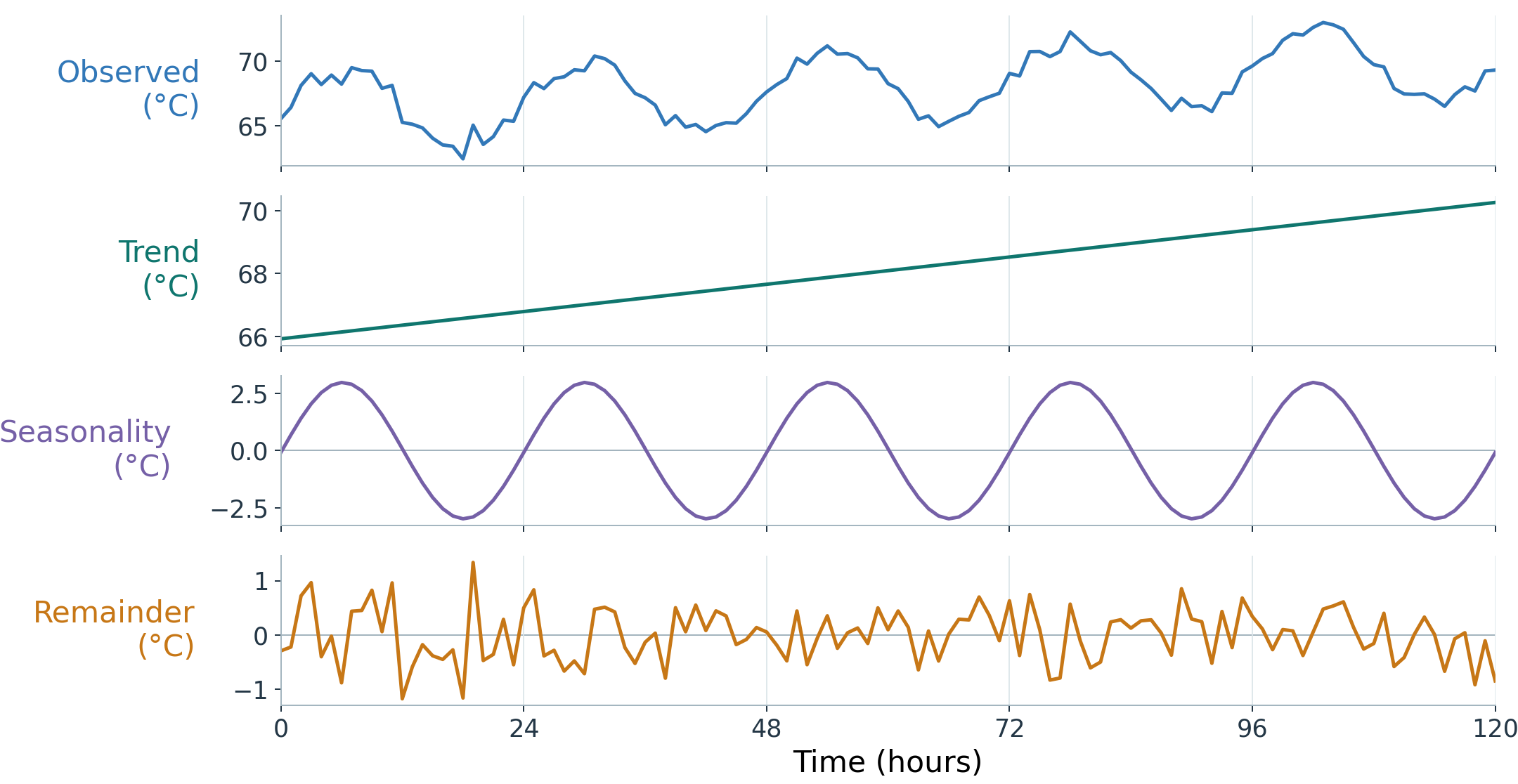
This is the same temperature series, now split into its three parts. All panels share the same time axis.

Figure 3. Additive decomposition of the temperature series from the earlier graph.

The remainder is not just noise: it can also hide unusual events, or patterns the split missed.

Read the panels from top to bottom. The observed line is identical to the earlier raw-series graph. The trend shows the overall rise; seasonality shows a daily cycle; the remainder shows what those two components do not explain. The vertical scales differ and are labeled in degrees Celsius, so compare tick values rather than apparent line height. Negative seasonal or remainder values are adjustments relative to the trend, not negative absolute machine temperatures. The generator fits a linear trend and a 24-hour sine/cosine pattern by least squares to the synthetic observations, then computes the remainder as observed minus the two fitted components. This is a simple illustrative additive decomposition, not an STL result or evidence about a real machine. The added random variation is known only because we generated the example; a remainder from measured data must be inspected before describing it as noise. This plot describes the observed history retrospectively. In forecasting evaluation, estimate decomposition and preprocessing using only data available at the forecast origin.

I.A) Understanding Time-Series Data Lags: How Past Readings Help Forecasting

Machine temperature often changes gradually, so a recent reading can help predict the next one. A relationship between readings at different times is called temporal dependence.

A lag tells us how far back a reading is from the value we want to predict.

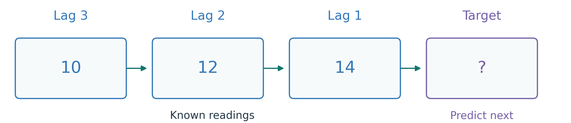
Predict the next reading from 10, 12, 14: lag 1 is 14; lag 2 is 12; lag 3 is 10.

Figure 4. Count lags back from the value being predicted.

Quick question: once 17 arrives, what are lags 1 and 2 when predicting the next reading?

Use the same target-relative lag convention as the later training table. For the next target after 17, lag 1 is 17 and lag 2 is 14. The timeline defines positions; three values do not establish statistical dependence. Autocorrelation measures linear relationships at a chosen lag and remains optional detail in the student notes. Temporal dependence may be nonlinear, seasonal, or associated with a trend. Test the usefulness of lag inputs on later data.

I.B) Defining the Forecast Choosing the Lookback Window and Forecast Horizon

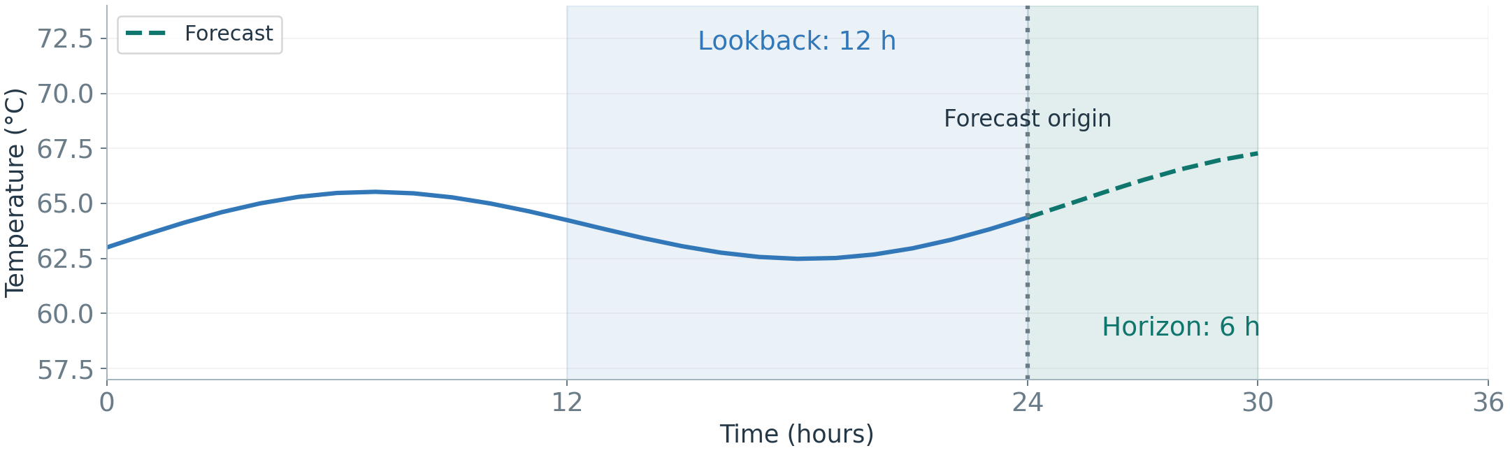
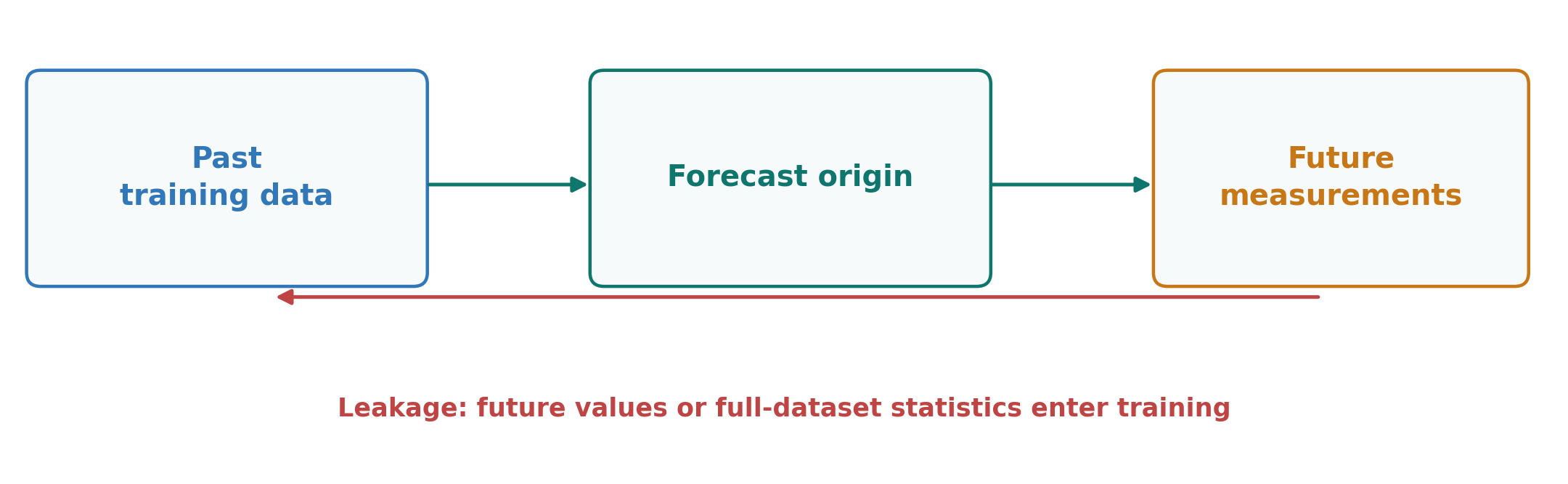
Forecasting uses information available now to estimate future observations. The forecast origin is the moment the forecast is made.

• Lookback window: the history supplied to the model.
• Forecast horizon: how far ahead we predict.

Example: use the previous 12 hours to predict the next 6 hours of machine temperature.

Figure 5. History ends at the forecast origin.

The forecast origin is the time the forecast is made. At hour 24 the future target readings are unavailable. Choose horizon from the decision: an operator reacting next hour and a planner scheduling tomorrow have different requirements. A longer lookback is not always more useful.

I.B) Defining the Forecast Choosing the Variables and Prediction Steps

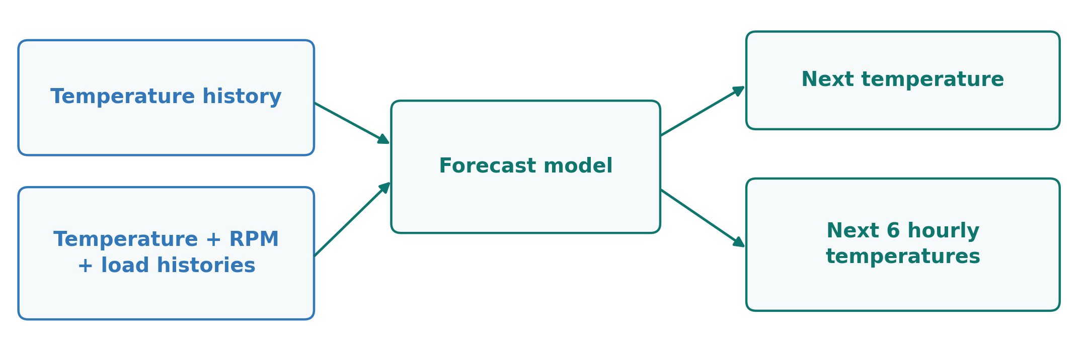
• Univariate: forecast a variable from its own history.
• With covariates: add related inputs, such as past RPM or a known future load schedule.
• Joint multivariate forecasting: forecast several related variables together.

One-step / multi-step means one future reading / several. Reusing predictions as future inputs can accumulate error.

Figure 6. Input choice and forecast horizon are separate decisions.

The slide distinguishes adding covariates to a single target from forecasting several targets jointly. Some sources use multivariate more broadly for any model using several variables. Multi-step forecasts can be generated together or by repeatedly feeding predictions back into a one-step model, which can accumulate error. A planned load schedule can be a known future input. Actual future load is unavailable unless known in advance.

I.C) Forecasting Methods How a Model Learns to Forecast

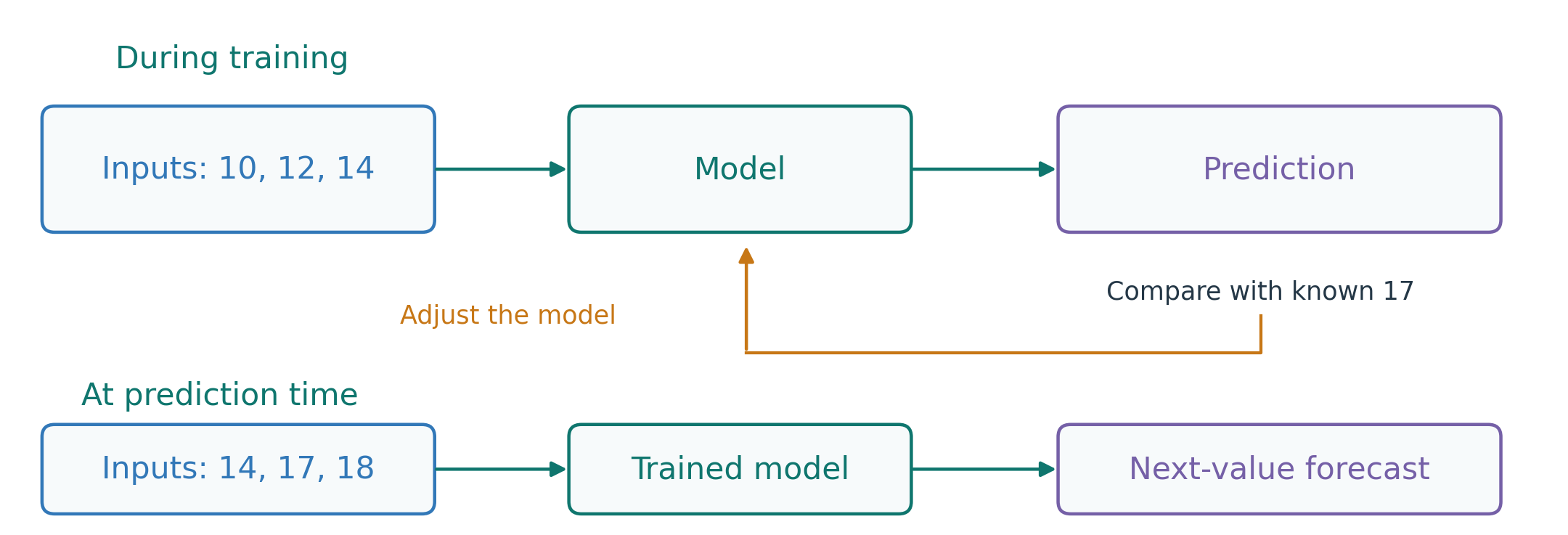
A model is a rule or learned relationship that turns inputs into a prediction.

• Inputs, or features: information we provide, such as three past readings.
• Target: the next reading we want to predict.
• Training: use past examples with known targets to adjust the model.
• Prediction: apply the trained model when the next target is still unknown.

Figure 7. Training uses known outcomes; forecasting estimates an unknown outcome.

Training adjusts model settings, often called parameters or weights, by comparing predictions with known targets. Prediction applies what has been learned to new inputs. The illustration does not prescribe a particular learned forecast or claim that one example is enough to train a model. A fixed rule, such as the naive forecast next, does not need learned parameters.

I.C) Forecasting Methods Comparing Forecasting Approaches

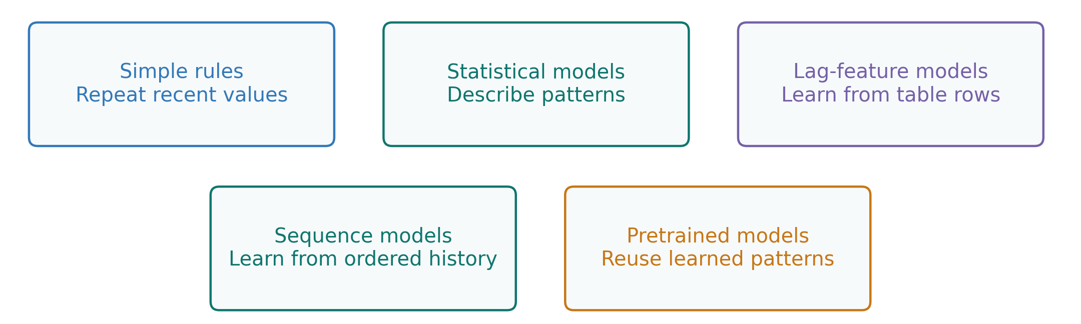
We can forecast the same target in several ways. The difference is how each approach uses history.

A baseline is a simple method used for comparison. Start there, then test whether a more complex method improves the forecast.

Figure 8. Alternative forecasting approaches, not steps in a required pipeline.

For each approach, ask: what history does it use, and does it beat the baseline?

This is a conceptual progression, not a strict historical timeline or claim that each family replaces the previous one. Lag-feature machine learning is often competitive for structured data. Sequence and pretrained models may reduce some feature design but add data or compute requirements. We will focus on mechanisms, not a catalog of architectures.

I.C) Forecasting Methods Naive Forecasts: Setting a Baseline

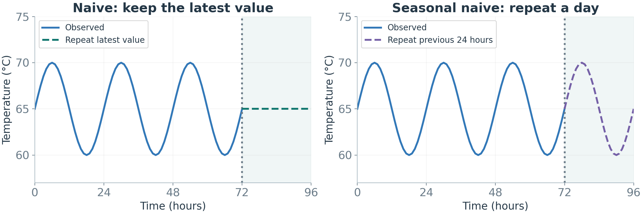
Naive: the next value equals the latest observation. Seasonal naive: repeat the value from the corresponding point in the last cycle. In decomposition terms, it reuses the seasonal pattern.

Fast and transparent, but unable to anticipate a new trend or operating regime.

If a complex model does not beat these baselines, reconsider its value.

Figure 9. Repeat the latest reading or the last known cycle.

The seasonal panel uses hourly observations with a 24-hour cycle. Repeat the value from the same hour on the previous day. Make the seasonal interval explicit and evaluate using the same horizon and data split as the proposed model.

I.C) Forecasting Methods Smoothing: Estimate the Recent Level

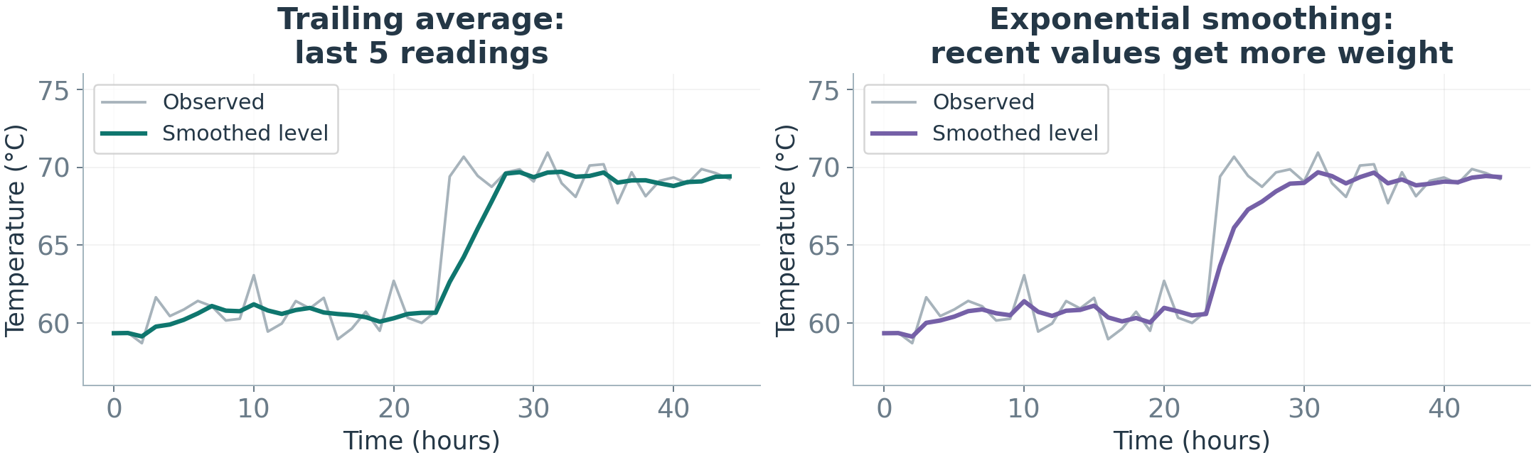
We want an estimate of the current level that smooths short-term fluctuations.

• Moving average: average the latest few readings.
• Exponential smoothing: combine the previous level and the latest reading using weighted averaging.

Example: previous level 70°C, new reading 80°C. Give the new reading 20% weight: 0.8\times70+0.2\times80=\mathbf{72}°C. Use 72°C as the next forecast.

Figure 10. Smoothing reduces short-term variation but responds after a change.

A larger weight reacts faster, but also follows more of the short-term variation.

The plotted lines are smoothed levels after observing each reading, not forecasts of that same reading. The forecast for y_t uses the level estimated at t−1. After observing y_t, the forecast for y_(t+1) uses the updated level at t. Holt smoothing adds trend; Holt-Winters adds seasonality. These are names for further reading, not new methods to teach here. A trailing moving average is a simple smoothing baseline; it is not the moving-average error component in ARIMA. Explain that noise reduction trades off against responsiveness.

I.C) Forecasting Methods Before ARIMA: Does the Pattern Stay Stable?

The next method, ARIMA, needs reasonably stable relationships in the series it models.

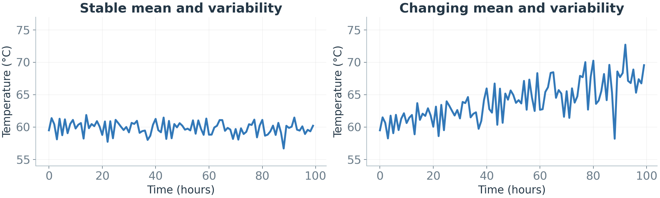
Stationarity means the average, spread, and relationships at a fixed time gap stay stable over time.

Figure 11. A stable level and spread on the left; a changing level and spread on the right.

Differencing stops looking at the value itself and looks at how much it changed: \Delta y_t=y_t-y_{t-1}.

Example: 10, 12, 14, 16, 18 keeps rising. Its changes are 2, 2, 2, 2: a stable pattern. The trend is gone.

Differencing can reduce a trend. It does not fix every type of change.

This is an intuitive description of weak stationarity. Its formal conditions are constant finite mean and variance, with covariance depending only on the time gap. The graphs illustrate mean and spread; they cannot prove stationarity. Explain differencing verbally: instead of asking what the temperature is, ask how much it changed since the previous time. From 10 to 12 it increased by 2, from 12 to 14 by 2 again, and so on, so the differenced series 2, 2, 2, 2 is stable even though the original keeps rising. That is exactly why differencing helps before ARIMA: it can remove a changing level and reveal a stable pattern underneath. Differencing does not necessarily stabilize variance. Stationarity is not a universal prerequisite for all forecasting methods.

I.C) Forecasting Methods ARIMA: Combine History and Past Errors

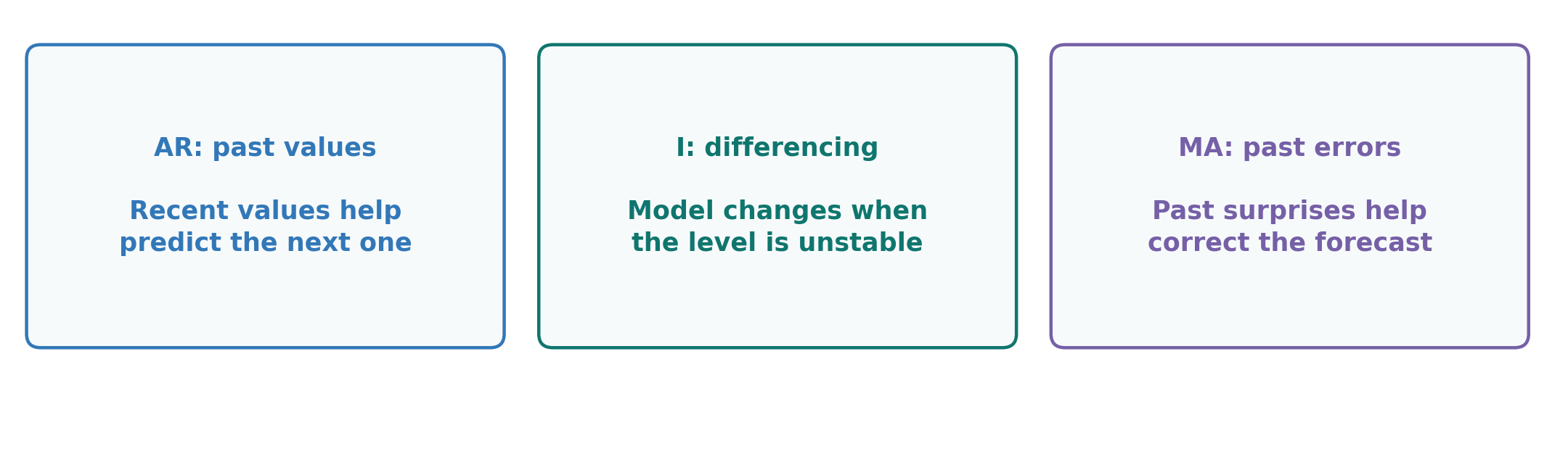
ARIMA combines past values, changes between readings, and past forecast errors.

Figure 12. ARIMA combines past values, differencing, and past forecast errors.

ARIMA(p,d,q): three numbers, one per ingredient.

• p: how many past values to use. This is the AR part.
• d: how many differencing steps. This is the I part.
• q: how many past prediction mistakes to use. This is the MA part.

A past prediction mistake, or residual: forecast 70, actual 72, a miss of +2.

ARIMA(2,1,1) differences the series once, then models the differenced series using two past lagged values and one past residual.

Expand ARIMA as autoregressive integrated moving average if needed. The explicit ARIMA(1,1,1) equation with its coefficients is written out and explained in the lecture notes; on the slide, p, d, q map one-to-one onto the three figure boxes. Past errors are weighted using learned coefficients; a positive error does not always imply an upward adjustment. The differenced series should have reasonably stable behavior. Seasonal versions and order selection are further reading, not required derivations here.

I.C) Forecasting Methods Lag Features: Turning History into Training Examples

A training example pairs available history with the value that came next. Lags are counted back from that target, just as in the earlier timeline.

Try it: for 10, 12, 14, 17, 18, use three past readings to predict the next one.

Table 1. Each row is one past forecasting example.

Lag 3	Lag 2	Lag 1	Target
10	12	14	17
12	14	17	18

Once 18 arrives, the next input row is 14, 17, 18. Its target is still unknown.

A model learns a relationship between the input columns and the target column.

Let students construct the two rows before discussing the answer. Linear regression and tree-based models can use such tables; there is no need to introduce their full taxonomy here. Rolling summaries use only available history. Calendar information can include hour or weekday. Lags preserve the position of past readings even when a model processes them as table columns.

I.C) Forecasting Methods Sequence Models: Learning from Ordered History

Keep the same task: use 10, 12, 14 to predict the next reading.

A sequence model learns from readings in time order. It can learn patterns across a longer history instead of relying only on summaries we chose.

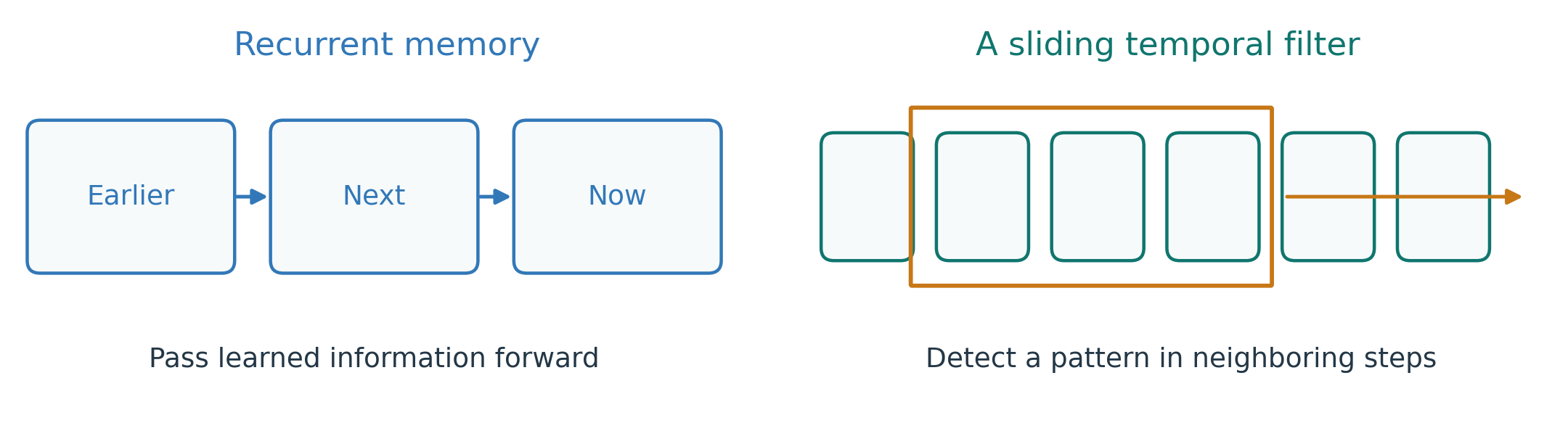
• Recurrent neural network (RNN): update a learned memory as each reading is processed.
• Temporal convolution: move a learned filter across nearby readings to detect short patterns.

Figure 13. Sequence models can retain information over time or detect patterns in short windows.

Both approaches learn patterns in history to forecast the next reading.

A learned memory is a vector of numbers, not a literal record of every reading. LSTM and GRU are recurrent variants covered as optional terminology in the notes. A temporal filter combines neighboring values using learned weights. Lag-feature models also use ordered history encoded in their columns; sequence models provide a different way to learn from it, not a guarantee of superiority.

I.C) Forecasting Methods Attention: Connecting Distant Times

What if a useful pattern occurred one day ago, rather than in the latest few readings?

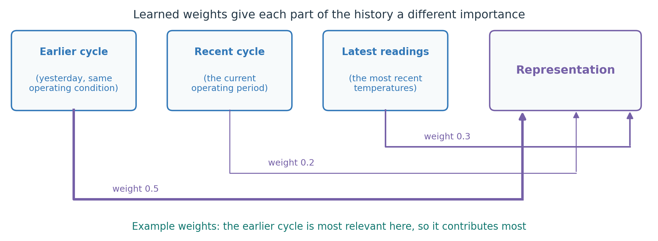
Attention learns how much information to use from different parts of the available history. A Transformer is a model that uses this mechanism.

Example: the model weights the earlier cycle 0.5, the recent cycle 0.2, the latest readings 0.3. The most relevant part contributes most.

Figure 14. Attention combines information from relevant parts of the observed history.

Attention can connect distant readings, but longer histories require more computation.

Unlike passing a state through every intervening step, attention can connect distant observed positions directly. Walk the figure: earlier cycle means yesterday at the same operating condition, recent cycle means the current operating period, latest readings are the most recent temperatures. Then explain the arrows: attention gives different importance, or weights, to these parts of the history. In the example the model decides earlier cycle 0.5, recent cycle 0.2, latest readings 0.3, so the earlier cycle contributes more because it is more relevant to the current situation. The weights are illustrative, not computed. Some forecasting Transformers group adjacent time steps into patches; PatchTST is one example, and its architecture is optional reading. Attention weights describe information weighting, not a proven causal explanation. There is no need to reteach Transformer internals.

I.C) Forecasting Methods Pretrained Models: Reusing Learned Patterns

We can also start from a model that already learned from many time series.

A pretrained model has learned settings, called weights, that we can reuse. A broadly reusable model is often called a foundation model.

Zero-shot forecasting: provide our machine’s history and request a forecast, with no weight update on our data.

Figure 15. Reuse a trained model, while still supplying the new series history.

The task stays the same. Compare its forecasts with our simple baseline on later readings.

TimesFM and Chronos are examples, retained in the lecture notes and references. Different model versions support different variables and forecast horizons. Zero-shot means no weight update on the target series, not no input history. Model reuse still requires checks for suitable inputs, domain fit, and independent evaluation.

I.D) Evaluating Forecasts Temporal Splits: Training on the Past, Testing on the Future

Before comparing methods, decide which data each method is allowed to use.

• Training: learn from the earlier readings.
• Validation: use later readings to choose the model and its settings.
• Test: assess the final choice on a period kept out of those decisions.

Figure 16. Learn first, choose settings next, and assess the final choice last.

Keep time order. Mixing past and future can give an overly optimistic result.

The mixed-color row illustrates random partitioning along the time axis. Repeated nearby patterns can make random evaluation misleading. A chronological test still needs correct feature construction and preprocessing. When using multi-step labels, keep training targets within the training period, and use a gap where overlapping targets would leak. For generalization to new machines, an additional machine-level split may be needed.

I.D) Evaluating Forecasts Leakage: Information Arrives Too Early

Data leakage: a forecast uses information unavailable at its forecast origin.

• A centered rolling mean averages readings before and after a time, including future values.
• A scaler adjusts feature ranges. Fitting it on all data uses future statistics.

Quick question (1 minute): can today’s prediction use tomorrow’s actual weather, or a weather forecast already issued today?

Figure 17. Future information must not enter past predictions.

Ask: tomorrow’s actual weather or tomorrow’s published weather forecast, which could be used today? Answer to the quick question: only the forecast already issued today. A forecast already issued today is available; tomorrow’s eventual observation is not. Similarly, planned load can be known in advance. Past history may legitimately provide context for validation and test predictions. The restriction is availability at the forecast origin, not an arbitrary ban on every input describing a future date.

I.D) Evaluating Forecasts Forecast Errors: Comparing MAE, RMSE, and MAPE

How far were our forecasts from the actual readings?

Actual energy: 10, 20, 30 kWh. Forecasts: 12, 18, 36. Error sizes: 2, 2, 6 kWh.

Table 2. Three ways to summarize the same forecast errors.

Measure	What it tells us	Formula	Calculation
MAE: mean absolute error	Average error size	\frac{1}{n}\sum_{t=1}^{n}\lvert y_t-\hat{y}_t\rvert	(2+2+6)/3=\mathbf{3.33} kWh
RMSE: root mean squared error	Gives large errors more influence	\sqrt{\frac{1}{n}\sum_{t=1}^{n}(y_t-\hat{y}_t)^2}	\sqrt{(2^2+2^2+6^2)/3}=\mathbf{3.83} kWh
MAPE: mean absolute percentage error	Average error relative to actual values	\frac{100}{n}\sum_{t=1}^{n}\left\lvert\frac{y_t-\hat{y}_t}{y_t}\right\rvert	(20+10+20)/3=\mathbf{16.7}\%

y_t: the actual value at time t; \hat{y}_t: its forecast; n: the number of forecasts, here 3.

Start with MAE. MAPE breaks near zero, so never use it on Celsius temperature.

MAE = (2 + 2 + 6)/3. RMSE = square root of (4 + 4 + 36)/3. MAPE = (20% + 10% + 20%)/3. Use energy here because it has a meaningful zero. Percentage errors on Celsius temperature are not meaningful. Ask which metric more strongly reacts to one very large error. Answer to the quick question: RMSE, because each error is squared before averaging. Compare the same target, horizon, and periods; MAE alone cannot compare variables with different units.

I.D) Evaluating Forecasts Walk-Forward Validation: Testing Several Forecast Origins

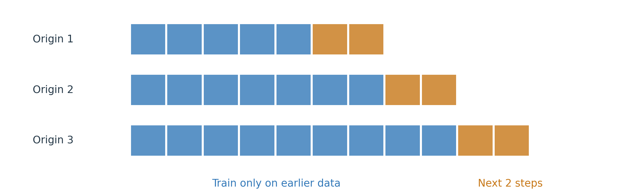
Walk-forward validation repeats forecasting at successive points in time.

At each origin: fit using earlier data, predict the required horizon, and record the errors.

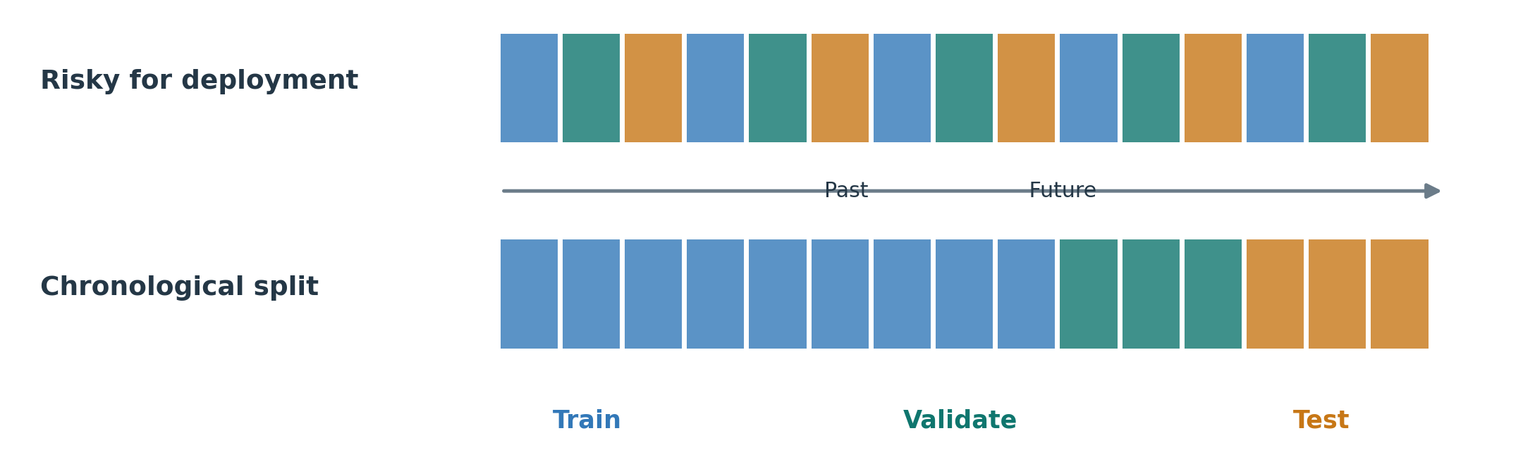
This tests performance across several periods, not only one convenient split.

Figure 18. Expanding training history with a two-step forecast horizon.

The blue blocks are training observations and orange blocks are the next two steps. Aggregate errors across origins and inspect each forecast horizon. A rolling training window can replace the expanding history. Keep a final test period separate from origins used to choose the model. Refit scalers and other learned preprocessing using only each fold’s training data.

I.D) Evaluating Forecasts Exercise: Walk Forward with a Naive Forecast

Series: 10, 12, 14, 17, 18. At each origin, predict that the next value equals the latest observed value.

Try it (3 minutes): fill in the three missing errors, then compute their MAE.

Table 3. Each forecast uses only the history available at that origin.

Origin	Forecast	Next actual value	Absolute error
After 12	12	14	…
After 14	14	17	…
After 17	17	18	…

We will solve it together. Notice what each forecast is allowed to see at its origin.

Answers: the absolute errors are 2, 3, and 1, so MAE = (2 + 3 + 1) / 3 = 2 units. The forecast after 17 can use 17 only because it has already been observed at that origin. Give students the full three minutes before solving. Then compare the three origins with the preceding walk-forward diagram. This is a fixed naive rule with an updated context, not a model fitted on future data. More complex models may also be refitted at each origin according to the deployment policy.

I.D) Evaluating Forecasts Prediction Intervals: Forecasting a Range

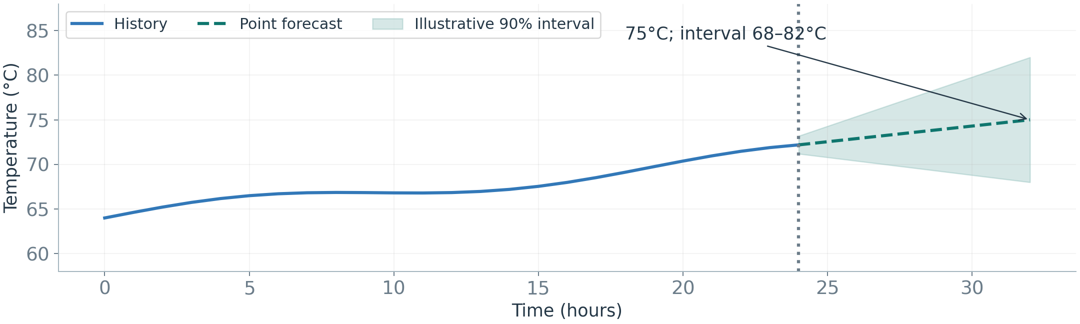
A prediction interval describes uncertainty about a future observation, not a safe operating range.

Example: 75°C, with an illustrative 90% interval of 68 to 82°C.

Observed coverage = test observations inside their intervals / test observations checked. If 90 of 100 are inside, coverage is 90%.

Check coverage and interval width together. Very wide intervals can cover almost everything yet offer little decision value.

Figure 19. Forecast uncertainty can grow with the horizon.

A calibrated 90% prediction interval should include about 90% of future observations over repeated comparable forecasts. It is not a guaranteed safe operating range, and is not a confidence interval for a model parameter. Ask whether the same action is appropriate for a narrow interval around 75 and a wide interval extending above an operational limit. Coverage should be checked on held-out periods and relevant operating conditions.

I.E) Distribution Shift and Adaptation Model Degradation: Monitoring Forecast Errors

A model performed well when we tested it. Will it stay accurate during daily use?

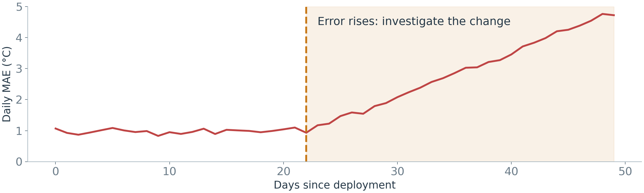
Model degradation means its predictions become less accurate over time. Compare forecasts with actual readings as those readings arrive.

Figure 20. An increase in forecast error is a reason to investigate.

Next question: did the operating conditions change, or did the machine behave differently under the same conditions?

The plot is an illustrative scenario, not a universal pattern. Error can rise because of concept drift, new input regions, sensor issues, or a poor model. Data-shift indicators can be useful when labels are delayed, but cannot alone prove that accuracy has fallen. Establish monitoring baselines and investigate the cause before updating.

I.E) Distribution Shift and Adaptation Covariate Shift and Concept Drift: What Changes?

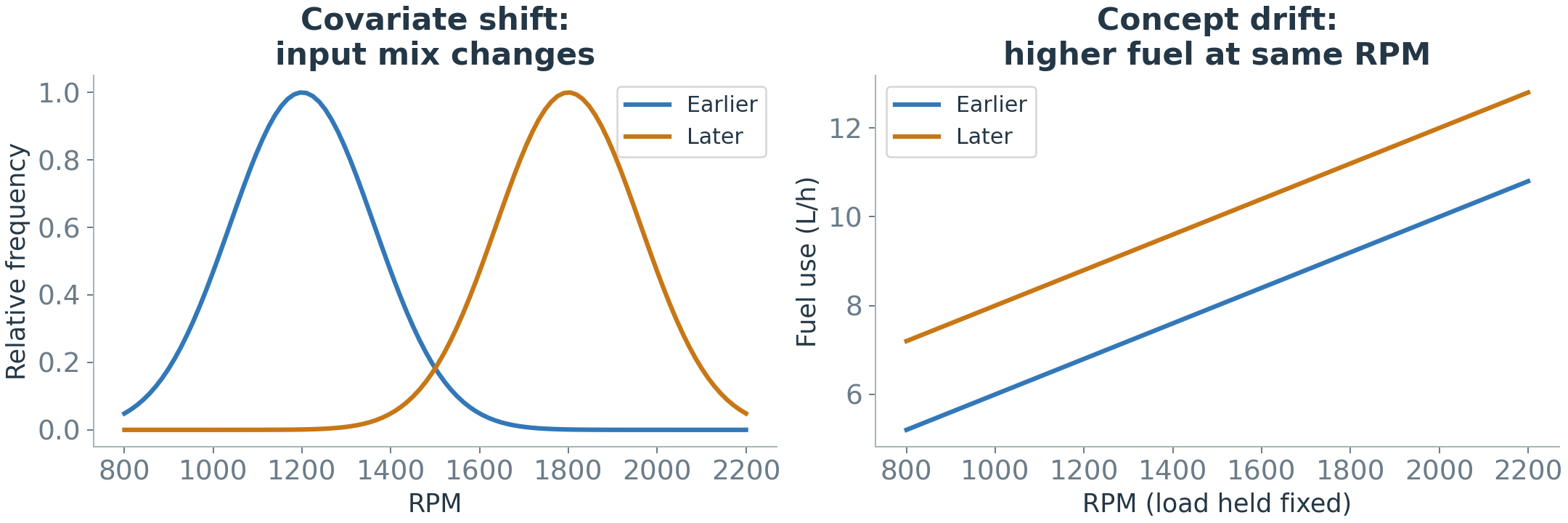
Rising errors can have different causes. Compare these two possibilities:

• Input change (covariate shift): more high-RPM operation; unchanged fuel use at the same RPM and load.
• Relationship change (concept drift): more fuel use at the same RPM and load.

Figure 21. Different inputs versus a changed relationship between inputs and output.

Check conditions and forecast errors before updating the model.

For readers of Gama et al., real drift changes P(Y|X); virtual drift changes P(X) without changing P(Y|X). Some authors use concept drift broadly for changes in the joint distribution. This lecture uses the narrower relationship-change sense and names the distinction explicitly. Non-stationarity is related but not identical: a time series can be non-stationary because its input mix or a predictable seasonal pattern changes. Machine aging, new operating policies, sensor replacement, and environmental changes can all change the observed data. In the left panel the input distribution changes. In the right panel the conditional relationship changes while load is held fixed. Both can occur together. A changing output average by itself does not tell us which happened. A predictable seasonal cycle is not automatically evidence that a learned relationship has failed.

I.E) Distribution Shift and Adaptation Drift Patterns: Sudden, Gradual, Incremental, and Recurring

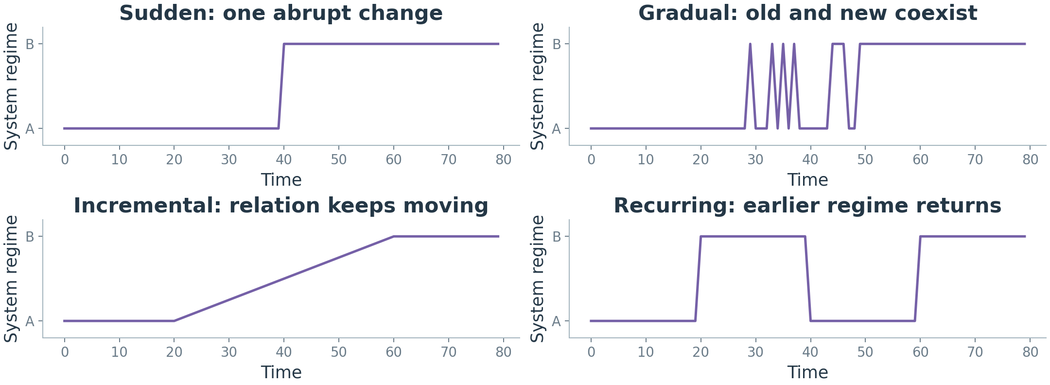
Sudden: abrupt replacement. Gradual: old and new behavior coexist during a transition. Incremental: the relationship keeps moving. Recurring: an earlier regime returns.

Quick question (1 minute): which panel fits a sensor replaced in one step? Which fits a machine that wears a little more each month?

Figure 22. Four schematic patterns of system change.

The vertical axis is a schematic regime indicator, not a measured sensor. A maintenance intervention can cause a sudden change. Gradual replacement differs from continuous movement: older and newer behavior can alternate during a transition. Gradual aging can move the relationship incrementally. Repeated operating regimes may recur; they need not be faults. Ask students to match one engineering example to a panel. Answer to the quick question: an abrupt sensor replacement matches the sudden panel; gradual wear matches the incremental panel.

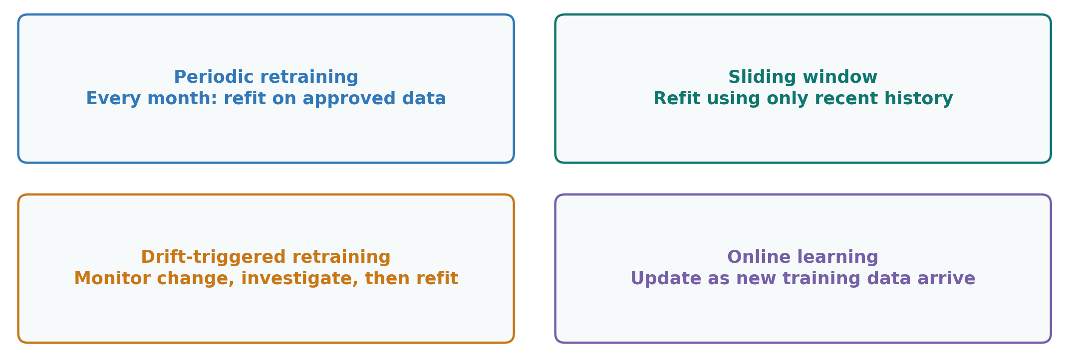
I.E) Distribution Shift and Adaptation Adaptation: Four Ways to Update a Model

• Periodic retraining: refit on a schedule.
• Sliding window: use only recent history.
• Drift-triggered retraining: investigate a detected change, then refit.
• Online learning: update incrementally as training data arrive.

Test each update on later data before relying on it. First investigate why performance changed.

Figure 23. Update strategies can be combined.

Periodic retraining is simple but can miss a change between scheduled updates. Sliding windows emphasize recent behavior but discard older examples, including rare valid regimes. Drift-triggered retraining requires reliable monitoring and can react to false alarms. Online learning updates incrementally when appropriate inputs and targets arrive; it is not required for every model. A sliding window describes which data are used, whereas periodic and triggered strategies describe when to update.

I) Forecasting From Prediction to Monitoring

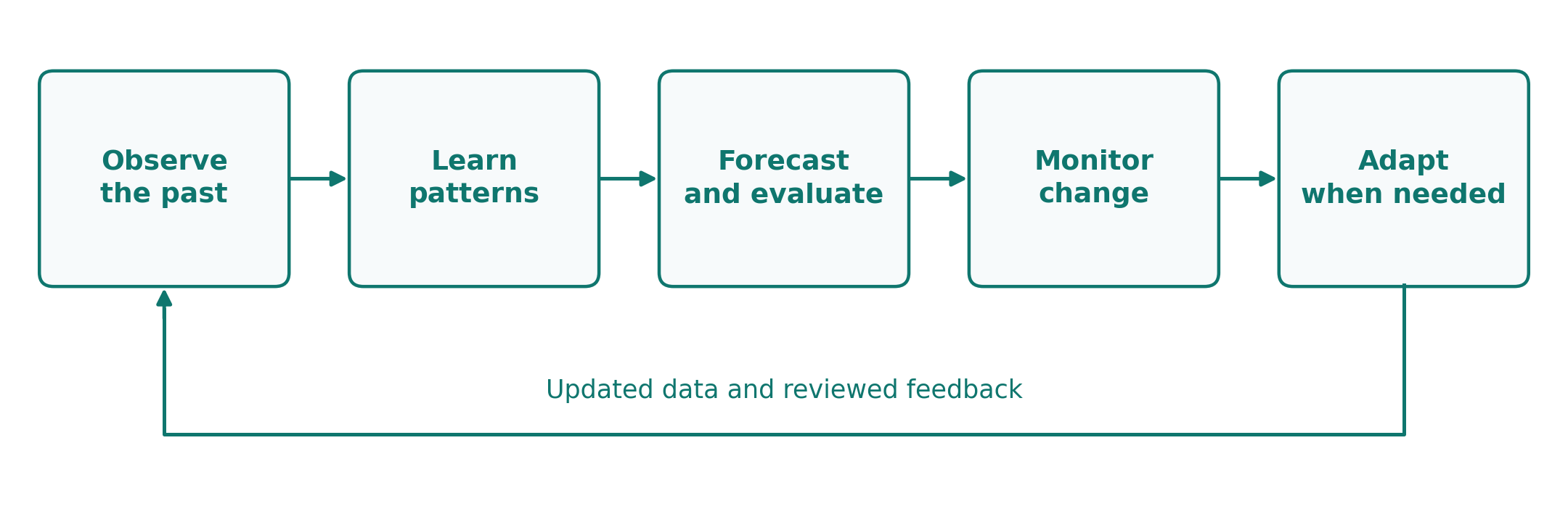
A useful forecast needs an appropriate baseline, honest evaluation, and monitoring.

Discuss: if errors rise after a sensor replacement, what would you check before retraining?

Forecasting asks what we expect next. Now we ask whether the observed behavior is unusual.

Figure 24. Forecasting is an ongoing process.

Allow about three minutes for discussion. Possible checks include calibration, units, timestamps, missing readings, and whether physical behavior actually changed. Retraining on a unit error would hide rather than solve the problem. Recap the lookback, horizon, chronological split, and baseline before the break.

BREAK

After the break: how can a model recognize unusual behavior?

II.A) Understanding Anomalies Anomalies: A Reason to Investigate

Part I taught us what to expect. Part II asks: what if the actual behavior does not match?

An anomaly is an observation or pattern that differs meaningfully from expected behavior. A temperature spike might reflect a fault, a sensor problem, or a valid operating event.

Anomaly detection tells us where to investigate. It does not establish the cause.

Figure 25. A deviation is evidence to examine, not a diagnosis.

Other examples include unusual transactions, network activity, heart rate, and energy use. Anomaly does not automatically mean failure, and some faults may produce no obvious anomaly. Expected behavior must be defined for a particular task and context.

II.A) Understanding Anomalies Normal References: Defining Expected Behavior

A normal reference is evidence we trust to describe expected behavior under the relevant operating conditions.

• Example: a period an engineer confirms was healthy, covering both low and high loads.
• Possible forms: limits, typical values, similar examples, or a forecast.
• Main risk: a reference with hidden faults or missing conditions can be misleading.

Without confirmed healthy data, a method still needs assumptions. For example, it may treat rare, isolated readings as unusual.

Ask first: what evidence tells us what normal behavior should look like?

A healthy period is a useful industrial reference, but unsupervised methods may lack this guarantee. Ask what happens if the reference contains only low-load operation. A reference also needs valid timestamps, units, and sensors. Normal is defined for the purpose of monitoring, not as an absolute property of a number. The closing point previews section II.B: supervised, one-class, and unsupervised settings differ exactly in where their definition of normal comes from, labels, confirmed healthy data, or a built-in rarity assumption.

II.A) Understanding Anomalies Detection Challenges: Rare Events and Changing Conditions

• Rare events: 990 normal examples may accompany only 10 anomalies.
• Few labels: engineers may not know which past readings were abnormal.
• Unknown events: future faults may differ from known examples.
• Noise: random variation can resemble a problem.
• Changing normality: a valid new operating regime may look unusual.

Why does this list matter? Every detection method in the next section is an answer to these difficulties. Each method builds its own picture of normal behavior in a different way, and then flags the readings that do not fit that picture.

Use the rare-event example to prepare for the later accuracy counterexample. Labels may be delayed until inspection, and even experts can disagree. Ask whether a detector trained on one speed should automatically apply at a different speed. This motivates contextual and multivariate detection.

II.A) Understanding Anomalies Anomaly Types: Points, Context, and Sequences

Before building any detector, know what shapes an anomaly can take.

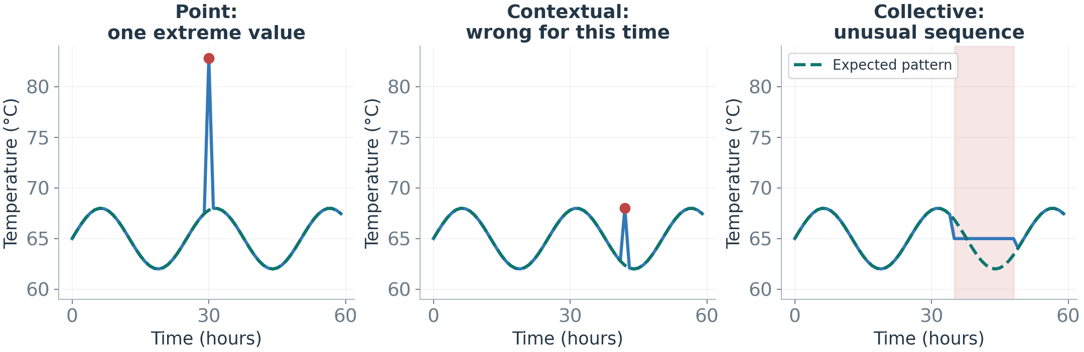
A point is unusual alone. A contextual anomaly is unusual for its time or condition. A collective anomaly is an unusual pattern across several readings.

Choose a representation that preserves the context needed to detect the problem.

Figure 26. Different anomalies require different evidence.

The contextual point is within the overall value range but too high for that part of the expected cycle. An alternative example is 25°C outdoors versus inside a refrigerator. In the collective example a flat segment replaces a normal oscillation; each value may be individually plausible. A pointwise threshold can miss that pattern.

II.A) Understanding Anomalies Multivariate Anomalies: Unusual Combinations

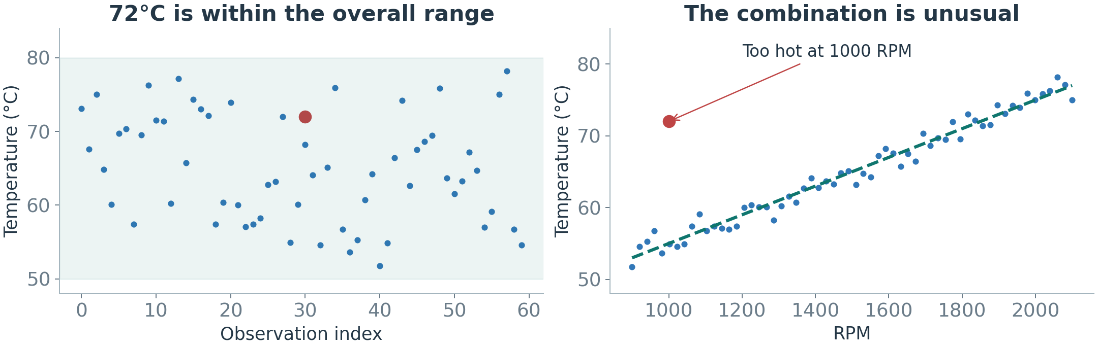
A temperature of 72°C can be normal at high RPM but unusual at 1,000 RPM.

Univariate detection examines one variable. Multivariate detection examines several variables and their relationships.

Separate sensor limits can miss an inconsistent combination.

Figure 27. The operating condition changes how a value is interpreted.

The same highlighted observation appears in both panels. The left panel shows temperature by observation index; the right panel adds RPM. The normal reference roughly follows temperature = 35 + 0.02 × RPM, so at 1,000 RPM about 55°C is expected. These illustrative values are not safe limits. More variables may still be needed, such as load and ambient temperature.

II.B) Defining Normal Behavior Learning Settings: What Labels Are Available?

A label records what an example represents, such as normal operation or a confirmed failure.

The labels available for training determine what we can teach a detector.

Table 4. Different training evidence leads to different learning tasks.

Setting	Available examples	What we teach the model
Supervised	900 normal, 100 failure labels	Distinguish the known classes
Normal-only / one-class	900 examples confirmed normal	Learn normal, flag departures
Unsupervised	1,000 examples, no labels	Search for unusual patterns

A method’s name does not determine its setting. What matters is the data used to train it.

Normal-only training is often called semi-supervised anomaly detection. Elsewhere semi-supervised commonly means mixed labeled and unlabeled data, so the slide uses the more transparent normal-only term. Supervised classifiers may miss unknown faults. Unsupervised methods often assume anomalies are rare or structurally different; they do not know that rare means faulty. The counts are hypothetical.

II.B) Defining Normal Behavior From an Unusualness Score to an Alert

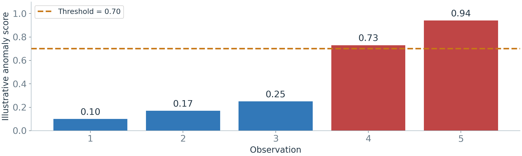
An anomaly score measures how unusual a reading or pattern looks to a detector. In this example, higher means more unusual.

A threshold is the cutoff for raising an alert: score > 0.70 → alert.

Figure 28. The two scores above the cutoff produce alerts.

A score of 0.94 is not automatically a 94% chance of failure. Some methods use different scales; a fixed rule may directly return yes or no.

The scores are invented and scaled to zero through one for illustration. A score of 0.94 does not mean a 94% probability of failure. Other methods produce unbounded scores. Rule-based methods may directly output a binary result. The threshold creates an operational decision from the model’s ranking.

II.B) Defining Normal Behavior What Does Each Detection Method Check?

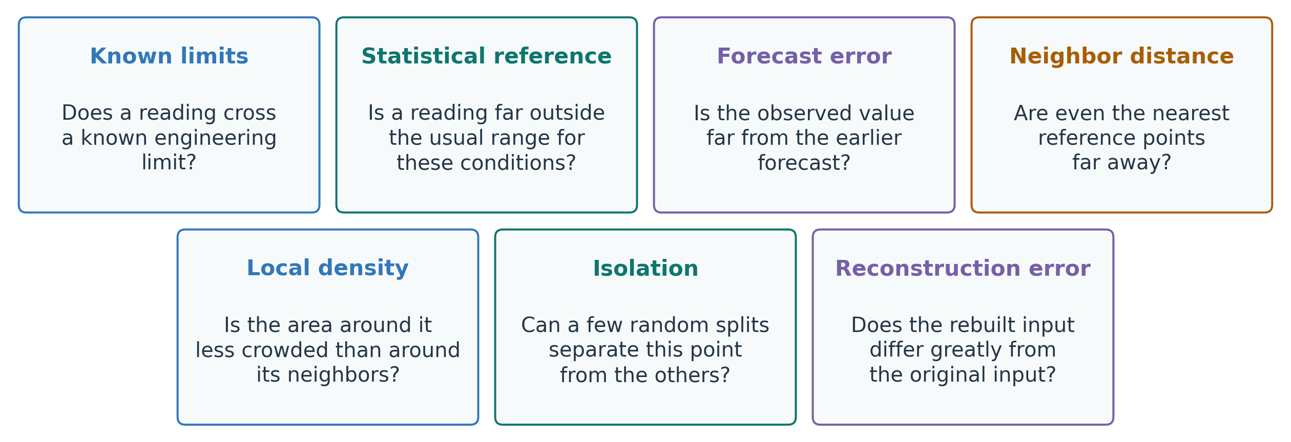
Each method checks a different kind of departure from expected behavior. These questions follow the order of the next method slides.

Figure 29. Questions used to check whether behavior is unusual.

Read left to right, then move to the second row. Known engineering limits and estimated statistical ranges are different references, so they have separate boxes. These checks can overlap: a forecasting model or an autoencoder can use several sensors together. Choose a check that retains the evidence needed to find the problem.

II.C) Anomaly Detection Methods Rules: Alert Outside a Known Limit

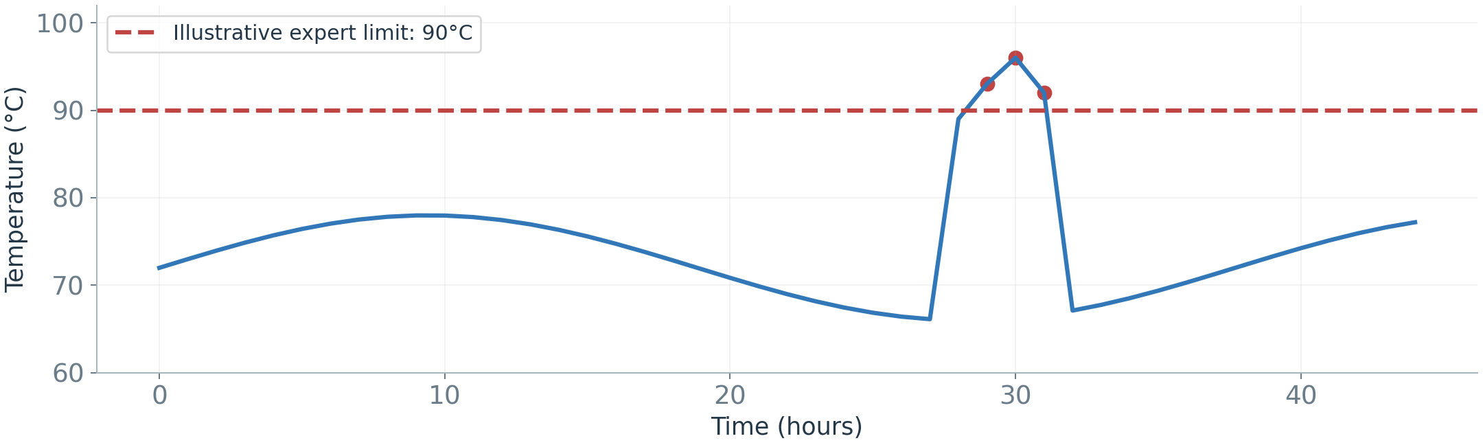
From the map: unusual means outside a limit. Example rule: temperature > 90°C → alert.

• Strength: clear, fast, and easy to explain.
• Limitation: a single limit may miss context or generate unnecessary alerts.

Use expert limits when they match the decision; do not treat them as a complete diagnosis.

Figure 30. An illustrative rule flags readings above a fixed limit.

The input is a temperature reading and the output is an alert decision. Here normal means within the selected rule, not necessarily healthy in every respect. The 90°C threshold is invented for this lecture. A real threshold must come from the equipment and use case. An anomaly model can complement rather than override an established safety rule.

II.C) Anomaly Detection Methods Statistics: Far from the Expected Range

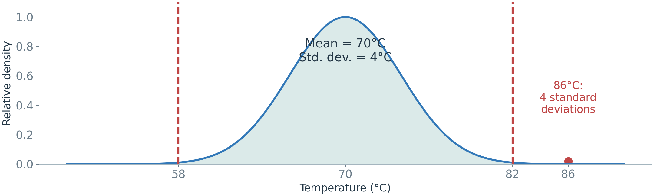
From the map: unusual means far from the expected range. Standard deviation measures spread around the mean of a suitable normal reference.

z=\frac{x-\mu}{\sigma}=\frac{86-70}{4}=4

x: reading; \mu: reference mean; \sigma: reference standard deviation. 86°C is 16°C above the mean, or four standard deviations.

Estimate the reference for comparable operating conditions. Lopsided (skewed) data and mixed regimes can make a single mean and spread misleading.

Figure 31. Mean ± 3 standard deviations is an illustrative rule.

The shown limits are 58 and 82°C. A three-standard-deviation rule is not a universal anomaly threshold. The familiar probability interpretation needs distributional assumptions. For skewed or contaminated data, quantiles, median-based measures, or an interquartile-range rule may be more useful. Estimate statistics without using the test period. If needed, describe the interquartile range as the distance between the 25th and 75th percentiles.

II.C) Anomaly Detection Methods Prediction: Compare Expected and Actual

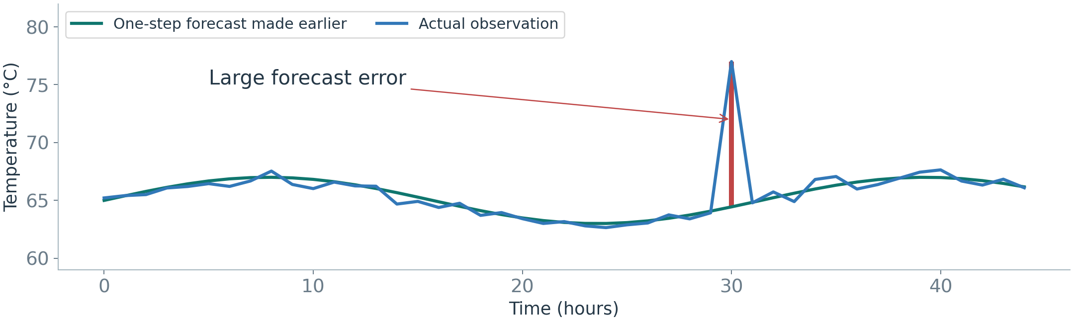
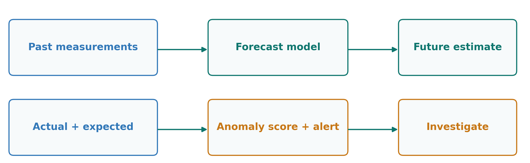
This connects detection to Part I: make a forecast, then compare it with the reading that arrives.

Forecast 70°C, actual 75°C: the absolute forecast error is 5°C. We can use that error as an anomaly score.

Figure 32. A forecast made earlier becomes the reference for checking a new reading.

Judge the error against usual forecast errors. A 5°C error is more unusual when typical errors are around 1°C than when they are around 5°C.

A poor forecast can cause a false alert. A large error alone does not prove a fault.

Use absolute forecast error as the first concrete score. Optionally normalize it by the estimated error standard deviation for comparable conditions: s=abs(actual-forecast)/sigma. For an absolute error of 5 and sigma 1, s=5; for sigma 5, s=1. Estimate sigma on earlier suitable data. This is an out-of-sample forecast error, unlike a retrospective decomposition remainder. Both compare data with an expected pattern, but they are not interchangeable quantities. A model that adapts too quickly may follow a developing fault.

II.C) Anomaly Detection Methods Neighbors: Is There Similar Data Nearby?

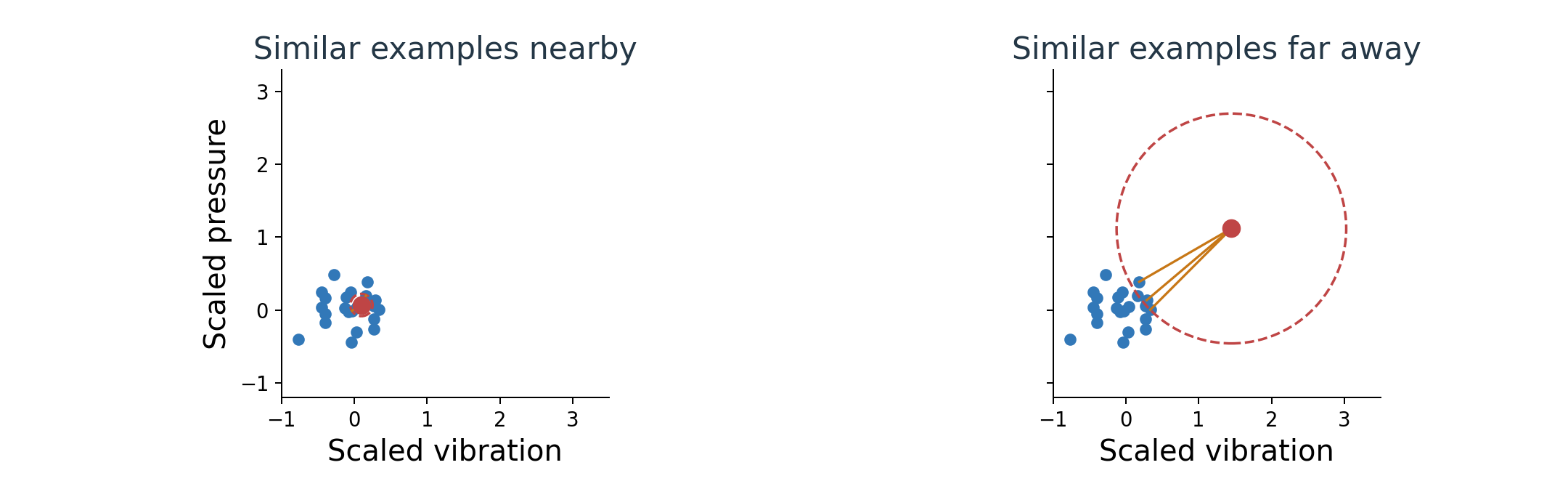
Idea: a reading looks unusual if similar examples are far away.

Each dot represents two measurements: blue = reference observations; red = a new observation.

k-nearest neighbors (kNN): choose a number of neighbors, k. Use the distance to the kth nearest reference point as the score. Here, k=3.

Figure 33. Compare the distance needed to reach three reference neighbors.

Make feature scales comparable first, so a large numerical unit does not dominate distance.

The query point is not part of the reference group. Dashed circles show distance to its third-nearest reference point. Larger distance gives a larger score. Choose k and a threshold using validation data. Distance provides a useful first intuition; the next slide addresses groups that have different densities.

II.C) Anomaly Detection Methods Local Density: Unusual Compared with Which Neighbors?

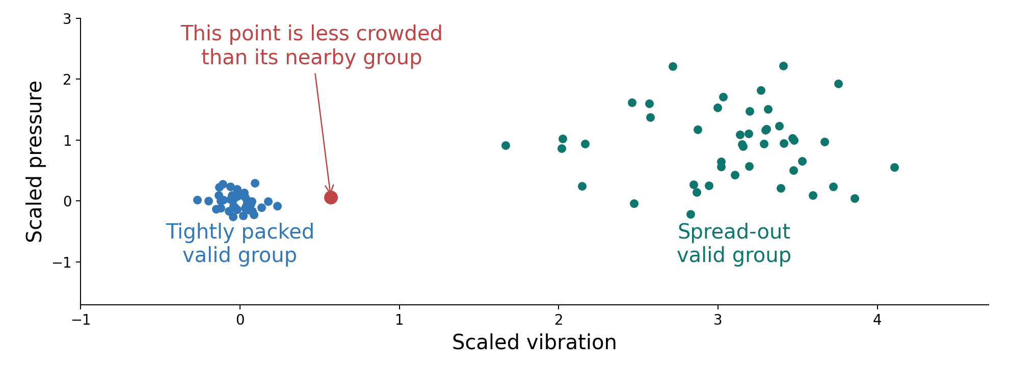
Distance alone can be misleading when one valid group is tightly packed and another is spread out.

Local Outlier Factor (LOF) asks: is this point in a less crowded area than its own neighbors?

Figure 34. A spread-out group can be normal; compare a point with its own neighborhood.

The comparison is local. A sparse group is not automatically a faulty group.

Density describes how tightly nearby examples are packed. LOF compares local reachability densities rather than raw global distances. A LOF value near 1 indicates similar local density, while a larger value indicates lower density than neighbors; the ratio and implementation details are optional notes. The figure is schematic and does not assign numerical LOF values. Validate neighborhood and scaling choices.

II.C) Anomaly Detection Methods Isolation Forest: Easy to Separate?

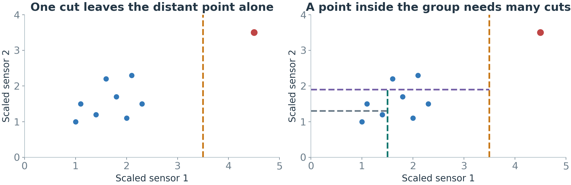
Idea: an unusual point is easy to separate from the rest.

Imagine cutting the data with random lines. Left: the red point is far from the others, so one cut is enough to leave it alone. Right: a blue point inside the group needs many cuts before it stands alone.

Isolation Forest repeats this with many random trees and averages: the fewer cuts a point needs, the more unusual it is.

It needs no labels and runs fast. Two limits: it does not see time order, and useless input features weaken it.

Figure 35. One illustrative tree; a forest repeats the random process.

The input is a feature vector and the score depends on average isolation path length. The diagrams show possible splits, not a guarantee that any single tree finds the anomaly. The red point is isolated by the first split; a blue point takes additional splits. Compared with neighbors, this approach does not compute density or nearest-neighbor distances directly. Scores still need a threshold and task-specific evaluation.

II.C) Anomaly Detection Methods Reconstruction: Can We Rebuild the Input?

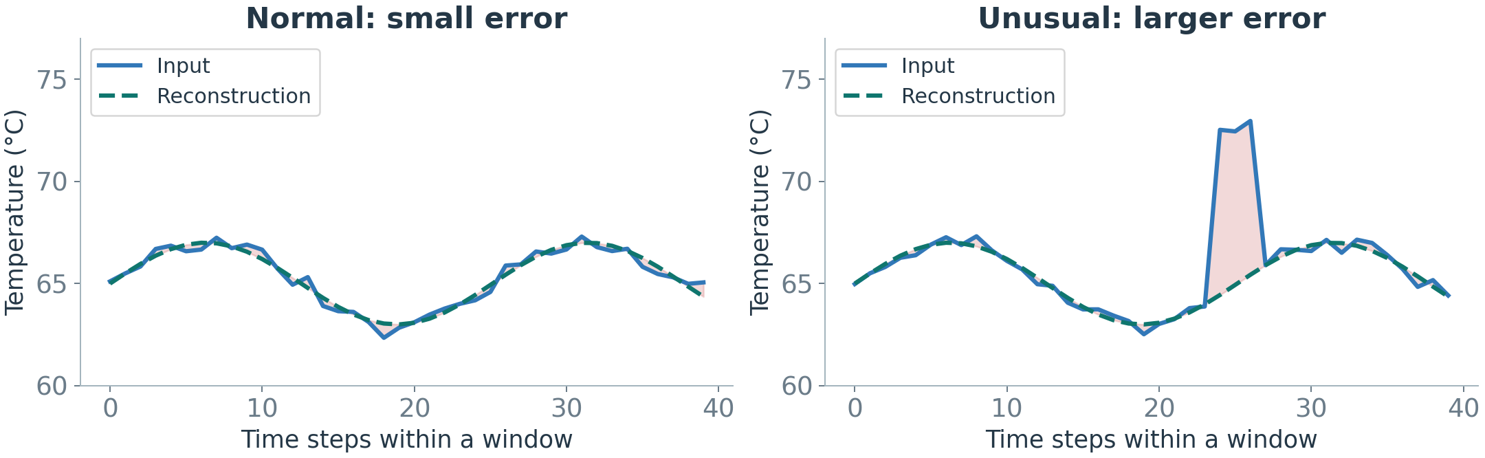
Reconstruction rebuilds a supplied input. Forecasting estimates a future reading.

An autoencoder learns to compress an input and rebuild it.

Train it on trusted normal examples. Then compare a new input with its reconstruction.

Figure 36. Compare the observed window with the model’s reconstruction of that same window.

Use reconstruction error as a score. Large errors suggest unusual patterns, but some anomalies can also be rebuilt well.

The encoder maps input values to a smaller learned representation; the decoder reconstructs the input. With input x_j and reconstruction xhat_j, a simple score is the sum of (x_j-xhat_j)^2 across time positions or sensors. Scale inputs so units do not dominate the score. Training on trusted normal examples helps define the reference but does not guarantee separation. Unlike forecasting, the supplied input includes the values being reconstructed.

II.D) Evaluating Anomaly Detection Evaluation Roadmap: Three Questions

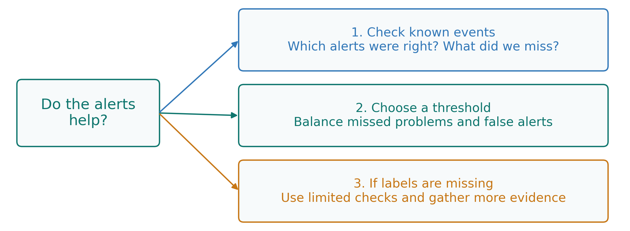
We have turned unusual behavior into alerts. Do those alerts help us find real problems?

We will answer three questions:

Figure 37. Evaluate whether alerts find problems, then choose settings that suit the task.

Use a labeled test period when available. Without labels, the evidence is more limited.

First motivate useful detection with the all-normal counterexample. Then define precision and recall and discuss threshold selection on validation data. If asked about long faults, note that one incident can span many readings and detection delay also matters; the lecture notes cover event-level evaluation in detail. Without independently identified events, expert review of alerts cannot measure how many events were missed. Rule-based detectors can directly produce alerts; other methods produce scores that require thresholds.

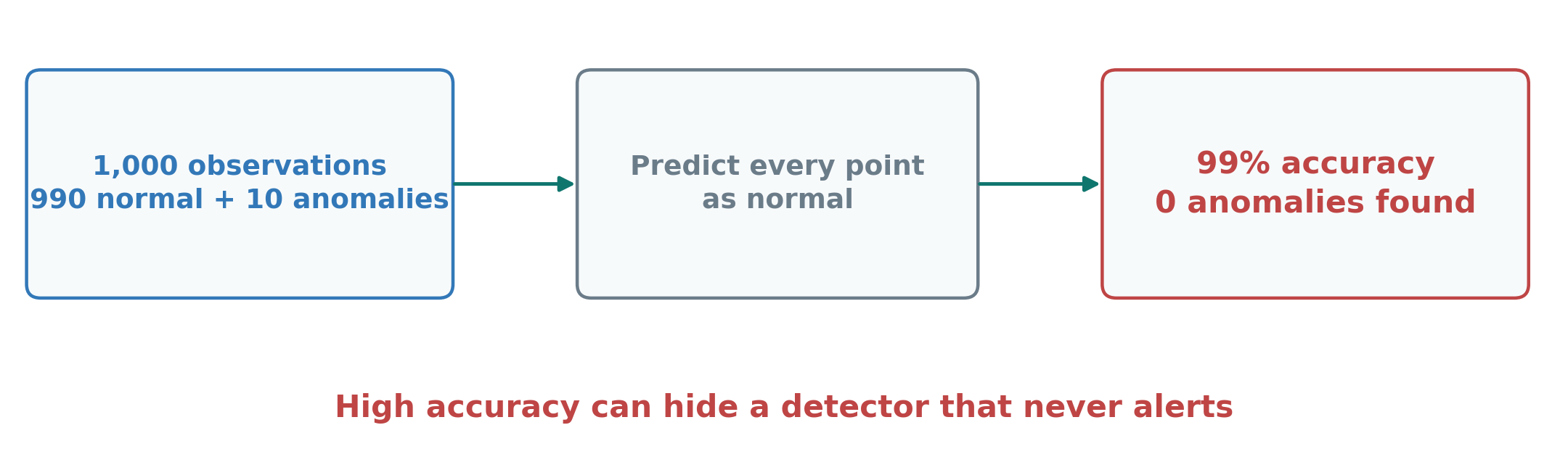
II.D) Evaluating Anomaly Detection Class Imbalance: Why 99% Accuracy Can Be Misleading

A detector predicts normal for every observation.

Its accuracy is 990 / 1,000 = 99%, but it finds none of the 10 anomalies.

Evaluate detected events and false alerts, not accuracy alone.

Figure 38. A high score can hide complete failure to detect anomalies.

Ask whether this detector would help an engineer. It never asks anyone to investigate. Because normal readings dominate, the accuracy score hides missed events. This motivates precision and recall rather than a change in the class definition.

II.D) Evaluating Anomaly Detection Precision and Recall: Counting Detection Outcomes

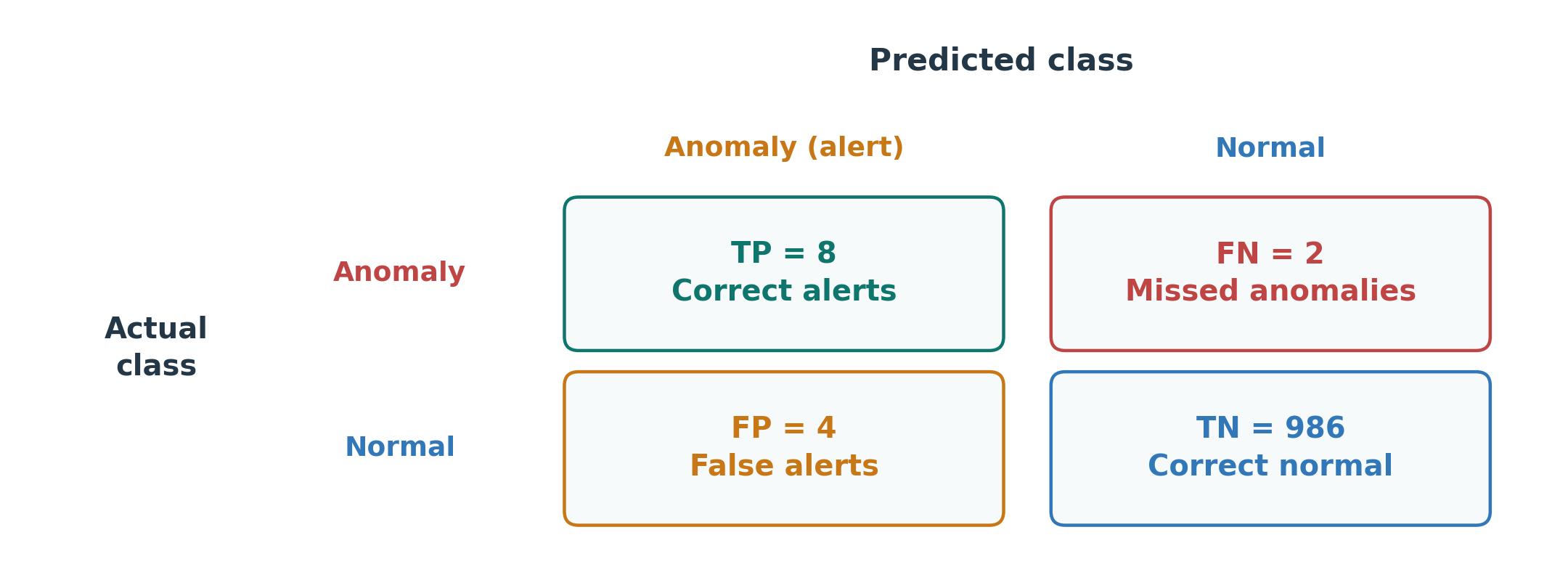
In a test period there were 10 anomalous readings. The detector raised 12 alerts: 8 correct and 4 false. It missed 2 anomalies.

• Precision: of all alerts, how many were correct? 8 out of 12 = 66.7%.
• Recall: of all anomalies, how many did we find? 8 out of 10 = 80%.

Figure 39. Correct alerts, false alerts, and missed anomalies answer different questions.

Precision describes alert reliability. Recall describes how many anomalies were found.

TP means true positive, FP false positive, FN false negative, and TN true negative. Precision=TP/(TP+FP); recall=TP/(TP+FN). The optional F1 score combines precision and recall with their harmonic mean: 2TP/(2TP+FP+FN)=16/22=72.7%. It does not represent all operational costs. Explain the two questions before discussing notation. Event-based counts need explicit grouping and detection rules.

II.D) Evaluating Anomaly Detection Threshold Selection: Balancing Misses and False Alerts

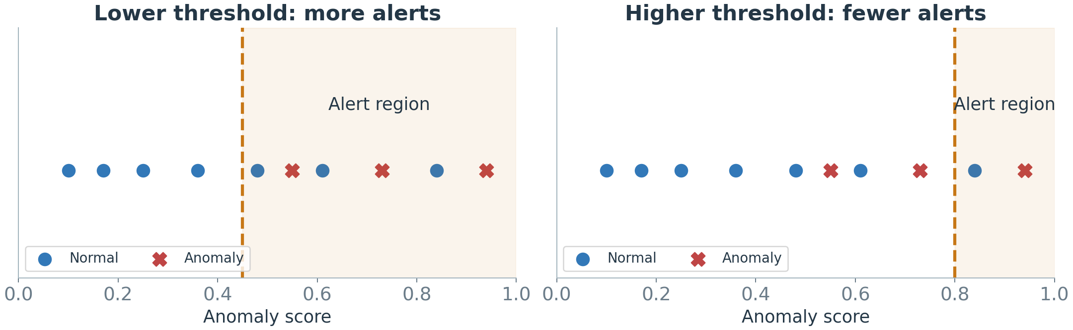
With a lower threshold, more readings raise alerts. This may catch more anomalies, but also creates more false alerts.

With a higher threshold, fewer readings raise alerts. Some anomalies may be missed.

Figure 40. Changing the threshold changes both correct detections and false alerts.

Choose on validation data: balance missed problems against false alerts and review capacity.

With only trusted normal data: a cutoff above 99% of those scores is one starting point. Check it later; it does not tell us how many anomalies will be missed.

Do not tune the threshold on final test data. A 99th-percentile threshold describes the reference scores and does not guarantee a future 1% false-alert rate. Recall requires independently identified anomalies, including missed events. Both points and grouped alerts should be assessed with the intended operational costs and capacity.

II.D) Evaluating Anomaly Detection Evaluation in Each Situation: What If Labels Are Missing?

Training labels and evaluation labels answer different questions. A detector trained without labels can still be checked against labeled test data.

Table 5. Match the strength of the conclusion to the available evidence.

Available test evidence	What we can check
Known anomalies and normal periods	Correct alerts, false alerts, missed anomalies, and detection delay
No reliable anomaly labels	Try artificial anomalies, ask experts to review alerts, and check behavior during trusted normal periods

Without known events, we cannot measure recall. Artificial anomalies test only the patterns we create; reviewed alerts do not reveal every missed event.

Use independently documented events whenever feasible, even if training was normal-only or unsupervised. Synthetic anomalies are limited sensitivity checks, not a substitute for real faults. Expert review can assess the inspected alerts but cannot by itself establish overall recall. Precision-recall curves and F1 are optional extensions in the student notes; they do not need to be additional slide prerequisites.

II.E) Monitoring in Practice Anomaly or Drift: Investigating Persistent Change

Evaluation used recorded data. Now the detector runs every day, and daily operation brings new questions.

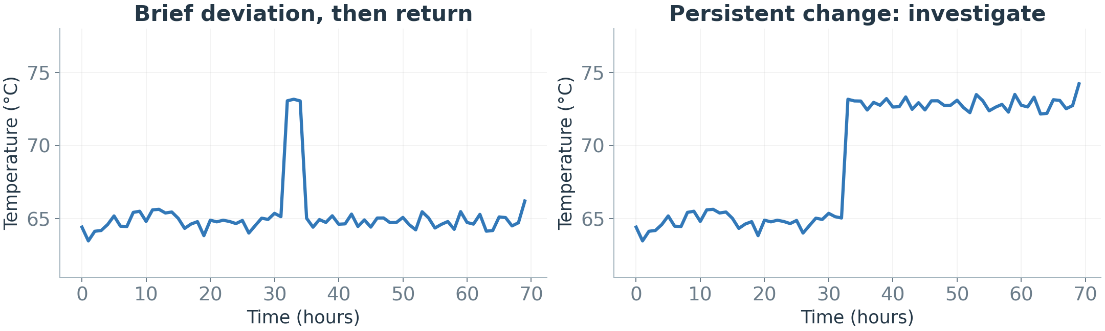
A brief spike may be an isolated anomaly. A persistent deviation may indicate a new regime, drift, a sensor issue, or an ongoing fault.

Duration is a clue, not a diagnosis. A persistent fault remains important even if it becomes common.

Before accepting a change as the new normal, check the operating conditions and whether the input-target relationship really changed.

Figure 41. A change in the trace does not reveal its cause.

This distinction intentionally avoids defining every anomaly as temporary or every persistent shift as benign drift. The left plot returns to its previous behavior. The right plot stays shifted, but the plot alone cannot distinguish calibration error, damage, or a valid policy change. The concept-drift definition from Part I concerns a changed relationship; additional input and target evidence is needed.

II.E) Monitoring in Practice Online Detection: Score Data as They Arrive

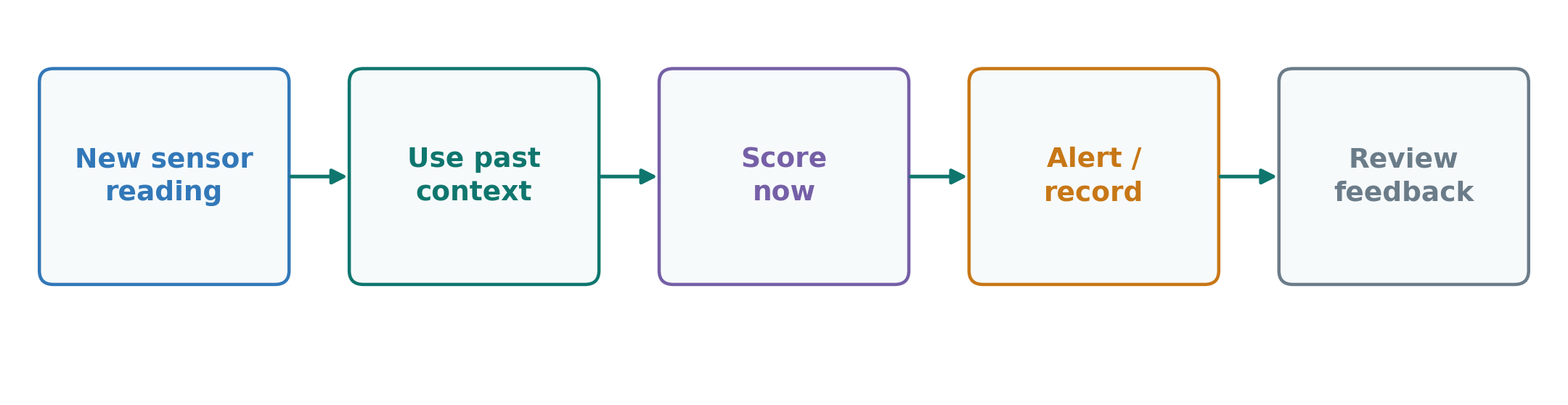
So far we scored recorded data. In operation, readings arrive one by one.

Offline: analyze a collected dataset later. Online: evaluate each new reading or short window as it arrives.

Meet the required response time while controlling false alerts. Online detection does not necessarily mean online model training.

Figure 42. Streaming evaluation can use a fixed or periodically updated model.

Inputs arrive continuously from manufacturing, infrastructure, network, or other monitored systems. A causal window contains only measurements already received. Windowing and alert-persistence rules can add delay. Decide what to do with late readings and missing sensors. Repeated alerts for one incident may be grouped for human review. Model updates remain a separate decision.

II.E) Monitoring in Practice Alert Explanations: Showing Evidence for Investigation

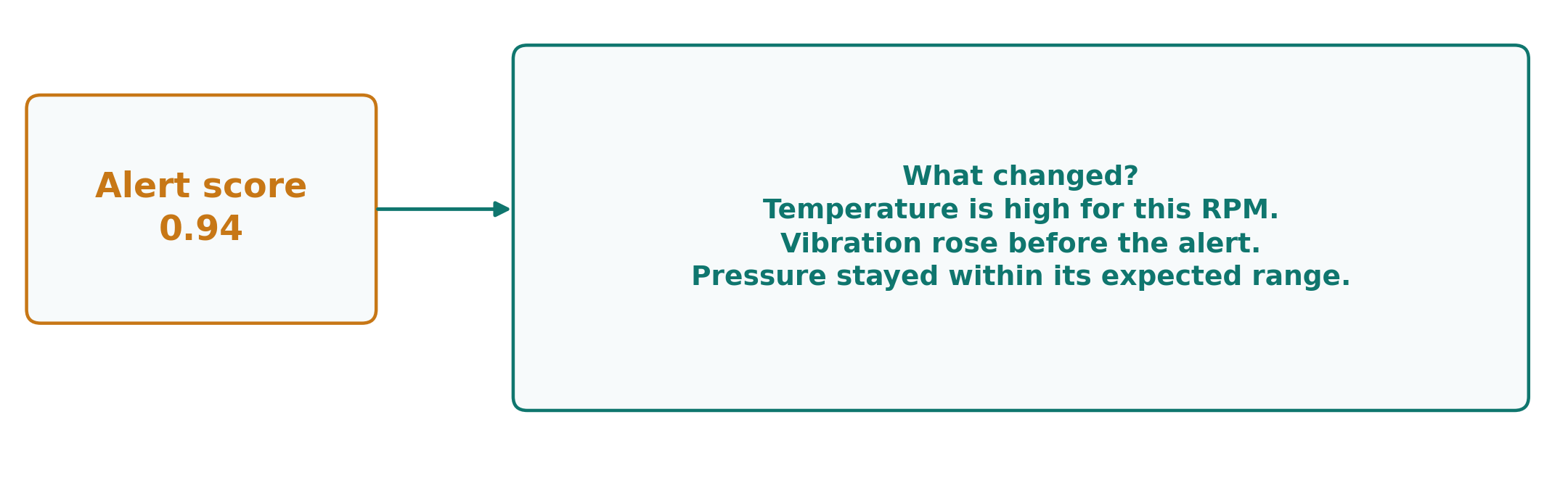
An alert has fired. What does the engineer see next?

For an alert score of 0.94, ask: what changed, when, and under which conditions?

Show expected versus observed behavior and the sensors contributing most to the discrepancy.

An explanation supports investigation; it does not prove a root cause.

Figure 43. Translate an alert into evidence an engineer can examine.

A sensor can have a large discrepancy because it is affected by the fault, not because it caused the fault. Comparing history, operating context, and related channels can guide inspection. No attribution algorithm is needed here.

II.E) Monitoring in Practice Human Review: Recording Findings and Improving Detection

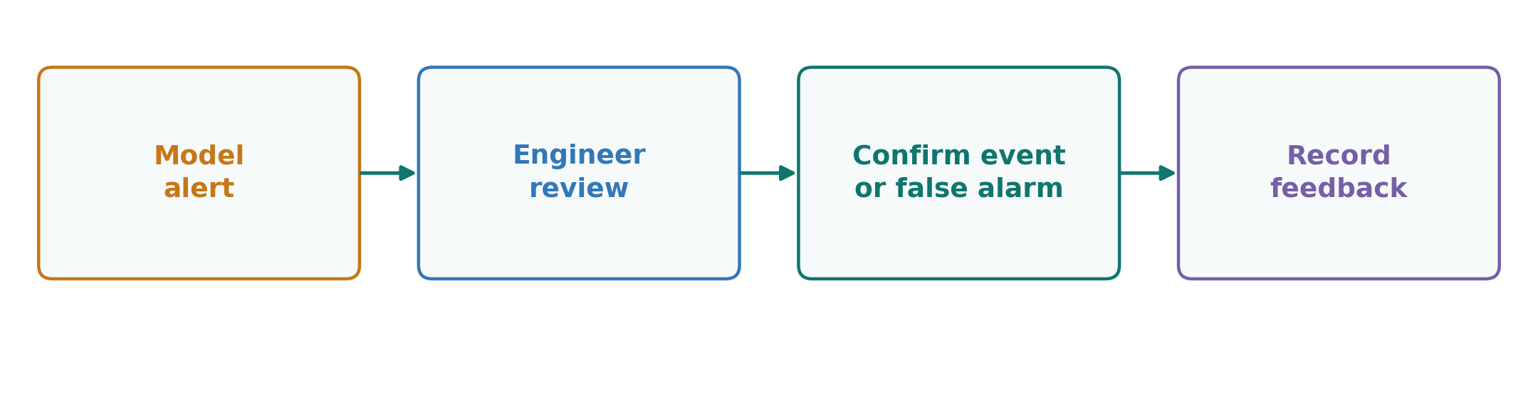
The last step of daily monitoring is human judgment. An engineer reviews the alert, checks context, and records what was found.

Useful feedback distinguishes a fault, a sensor problem, a valid event, and an unresolved case.

Use reviewed feedback to improve thresholds and training data. An unreviewed alert is not a confirmed anomaly label.

Figure 44. Detection and human review have different responsibilities.

Keep a record of reviewed examples and changes to the detector. Confirmation may take time, and different engineers may need consistent labeling guidance. The figure ends in recorded feedback; applying that feedback to training or thresholds should be an explicit validated update. Systems may take immediate protective action when required by the application, but anomaly scores alone do not specify that action.

II.F) From Detection to Decisions Method Selection: Choosing a Suitable Starting Point

Which method should you start with? Ask what evidence you have. Find your row, start there, then test on later data.

Table 6. Match the evidence you have with a starting method.

What you have	Start with	Be careful
Safe limits from engineering knowledge	A fixed rule	It cannot see context
Examples labeled normal and fault	A supervised classifier	New faults it has never seen
A stable, confirmed healthy period	Statistics: mean and spread	Conditions that change over time
Many trusted normal examples	Neighbors: kNN or LOF	Scale features, choose k carefully
Mostly normal rows, no labels	Isolation Forest	It cannot see time order
Trusted windows of normal readings	An autoencoder	It may rebuild anomalies well too
A forecast you can trust	Forecast error as the score	A poor forecast creates false alerts

These are starting points, not final answers. Whatever you pick, compare it with a simple baseline on the same later events.

This table is a practical starting point, not a universal ranking. A supervised classifier is also possible when representative normal and anomaly labels exist, as covered earlier. Ask students to choose one row for a machine with no confirmed failure labels but a documented healthy period. Evaluate the chosen method against a simple reference before adopting it.

II.F) From Detection to Decisions Detection, Diagnosis, and Prognostics: Different Questions

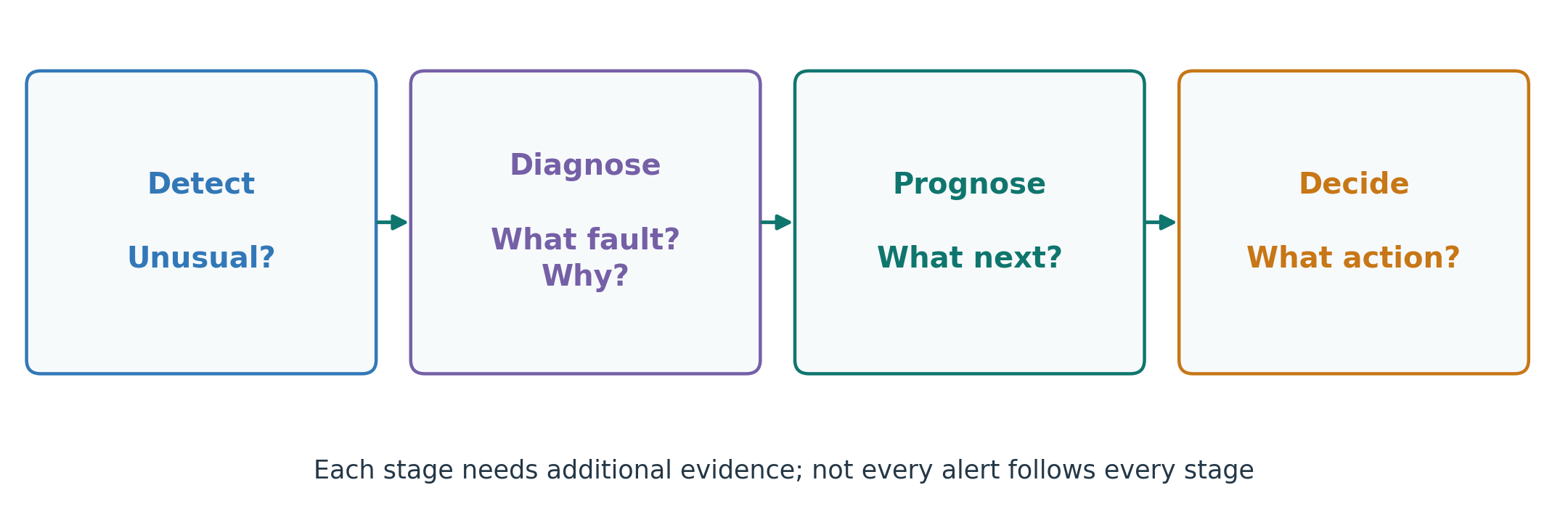
Detection found something. What happens after an alert?

• Detection: something differs from expectation.
• Diagnosis / root-cause analysis: what fault occurred, and why?
• Prognostics: how might the condition develop, or when might failure occur?

An action needs evidence, operating constraints, and human responsibility.

Figure 45. Later stages need evidence beyond an anomaly score.

Diagnosis can identify a fault category; root-cause analysis seeks the underlying cause. Prognostics may estimate remaining useful life, with uncertainty. Not every detected anomaly requires prognostics, and urgent protective action may precede a complete diagnosis. Present this as a possible workflow, not an obligatory sequence or an autonomous causal reasoning capability.

Week 4: Summary Expected Behavior Connects Both Tasks

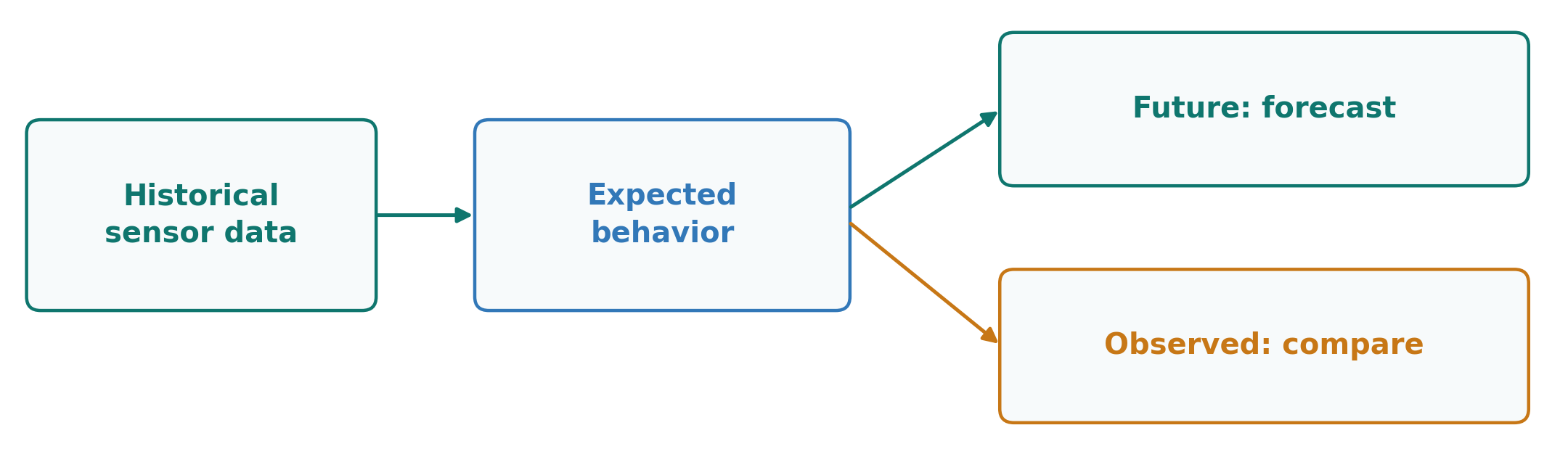
Forecasting: what should happen next? Anomaly detection: is what happened consistent with what we expected?

Use honest temporal evaluation, meaningful thresholds, and monitoring for change.

A prediction or alert is useful when it supports a better decision.

Figure 46. Two questions built on an appropriate expectation.

Ask students to state one reason a high anomaly score might not mean failure, and one way future information can leak into a forecast. Return to the opening questions. Accurate prediction is only part of the workflow: uncertainty, context, evaluation, and response determine its practical value.