Lecture 1 Notes: Overview of Applied AI
These notes follow the Lecture 1 slides in the same order. The section and subsection titles match the slide topics. Use the explanations to review each idea, and the review questions to check your understanding. A glossary and the two case-study references appear at the end.
What Is Applied AI?
Applied artificial intelligence (AI) uses AI methods to address practical problems. It connects a clear need, a suitable method, and a useful result. Training a model is one part of this work. Other parts include obtaining reliable data, evaluating results, and helping people use the output.
Consider a maintenance team that wants to reduce unexpected pump failures. An AI model could estimate failure risk from sensor measurements. The application also needs a way to collect those measurements, show warnings to a planner, and check whether the warnings lead to useful inspections. This example will connect the basic ideas throughout the lecture.
Lecture Roadmap
The lecture has three parts:
Basic concepts: AI, machine learning, and common tasks
Working systems: data, evaluation, and use in practice
Case studies:
- Engineering design case: completing a design with fixed requirements
- Engineering well-log case: estimating missing measurements
The cases show how a practical problem connects to its data, method, evaluation, and use.
1. Basic Concepts
What Can AI Systems Do?
Artificial intelligence is the field of building systems that perform tasks associated with intelligent behavior. These tasks include interpreting images or signals, making predictions, combining facts and rules, producing candidate outputs, and supporting decisions.
For example, a factory system might identify a defect in an image, assign a defect category, and recommend an inspection. These capabilities overlap; they are not separate requirements that every AI system must satisfy. An AI system can make mistakes, so its output needs evaluation in the setting where it will be used.
AI, Machine Learning, and Deep Learning
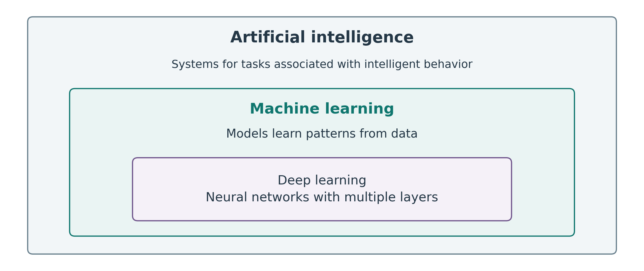
Machine learning (ML) is a part of AI in which models learn patterns from data. Deep learning is a family of ML methods that uses neural networks with multiple layers. A neural network is a model built from connected computational units whose adjustable parameters are learned during training.
AI also includes methods based on explicit rules. For example, a system can combine facts and written rules to draw a conclusion without learning from examples. Deep learning is useful for many problems, but it is not always the most suitable method. The choice depends on the task, the amount and quality of data, the computing resources, and the requirements for use and maintenance.
Rules and Learning From Examples
In traditional programming, a developer specifies how the system should process data. A simple pump-monitoring rule might raise an alert when temperature exceeds a set limit. This approach can be useful when the rule is clear and reliable.
In supervised learning, training examples contain both inputs and known answers. Past pump readings can be paired with records of whether a failure occurred within the next 24 hours. A learning algorithm uses these pairs to fit a model: a learned relationship between inputs and outputs. The result need not be a set of readable rules.
Not all ML requires a known answer for every example. For instance, unsupervised learning looks for patterns in data without supplied target labels. An application can also combine written rules and learned models.
Training and Inference
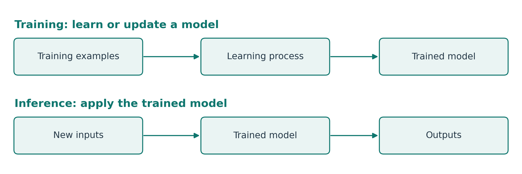
Training learns or updates a model from data. Inference applies a trained model to an input to produce an output. In the pump example, training uses past sensor readings and failure records. Inference uses recent readings to estimate a future failure risk.
Training may be repeated as more data becomes available or requirements change. Inference may happen immediately, such as when a new reading arrives, or in scheduled batches, such as a daily maintenance report. Training data is not automatically clean, and inference is not automatically fast; both require suitable preparation and engineering.
Common Tasks in Applied AI
A factory provides examples of several common tasks:
| Task | Purpose | Factory example |
|---|---|---|
| Regression | Predict a number | Estimate product strength |
| Classification | Assign a category | Label a product as defective or acceptable |
| Forecasting | Predict future values | Estimate next week’s electricity demand |
| Anomaly detection | Identify unusual patterns | Flag unusual pump vibration |
| Generation | Produce candidate outputs | Propose a component design |
| Optimization | Search for the best feasible option | Select operating settings |
These task descriptions can overlap. Forecasting a future numerical value is also regression. An inverse design application may generate candidates and then use optimization to choose among them. Optimization can use an AI model, but it does not require AI. An unusual observation is also not necessarily a fault: a change in operating conditions can produce an anomaly.
Define a Useful AI Task
A practical goal becomes easier to study when its output, time horizon, data, and user are explicit:
Estimate whether a pump will fail within the next 24 hours, using recent sensor readings, so a maintenance planner can prioritize inspections.
Quick check (1 minute): what task type is this, and what past records would be needed?
Suggested answer: this is a binary classification task: failure or no failure within the specified interval. It needs sensor histories and reliable failure times. At prediction time, only information already available may be used. The future outcome supplies a training label, not an input for inference.
Optional extension: what would change if the required output were “hours until failure”? This would be a regression task, and training would need suitable records of operating time and failure outcomes. Changing the output can change both the data requirements and the evaluation measures.
2. From a Model to a Working System
Connect the Output to a Decision

For the pump application, the model produces an estimated failure risk within 24 hours. The maintenance planner reviews the warning and decides whether to schedule an inspection. The intended value is fewer unexpected stops with a manageable inspection workload.
A prediction does not determine the action by itself. The planner also considers available staff, inspection costs, and the consequences of a missed failure. Other applications may support understanding through a report or explanation. In each case, identify who uses the result and how it helps.
The Applied AI Lifecycle
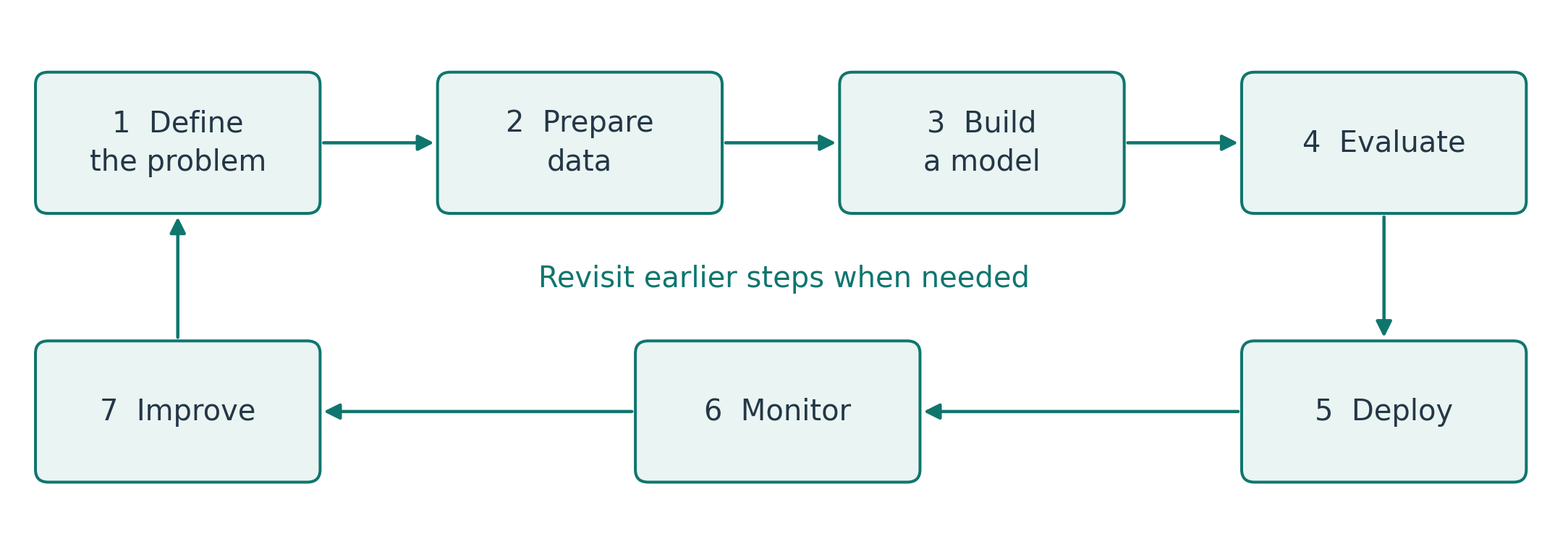
The lifecycle organizes the work into seven related steps:
- Define the problem: identify the user, desired output, and practical goal.
- Prepare data: collect, check, and organize relevant examples.
- Build a model: select and train a suitable method.
- Evaluate: compare results with a baseline and the application requirements.
- Deploy: put the model into the intended workflow.
- Monitor: check data, outputs, and practical performance during use.
- Improve: address problems and evaluate any changes before relying on them.
These steps are iterative. A weak result may reveal a problem with the data or task definition. After deployment, new equipment or operating conditions may change the data the model receives. Drift means a change in the data distribution or in the relationship between inputs and outcomes; it may, but does not always, reduce performance. Monitoring helps identify when further investigation or an update is needed.
What Data Does the Task Need?
Four questions help assess whether data is suitable:
- Features: which inputs are available? For a pump, these might include recent temperature, vibration, and load.
- Labels: which answers are known? In supervised learning, a label might indicate whether a failure occurred within the following 24 hours.
- Quality: are the records reliable? Incorrect timestamps or faulty sensors can make examples misleading.
- Coverage: which conditions are represented? Data from one pump or season may not represent all intended uses.
Labels apply to supervised learning; other approaches may use unlabeled data. A useful check is whether each proposed input will actually be available during inference. Data leakage occurs when information from outside the valid training or prediction setting enters model development or evaluation. For example, using a repair record written after a failure to predict that same failure would produce an unrealistic result.
Data Has Different Forms
Structured data is organized into defined fields, such as the columns of a sensor table. Unstructured data includes images, free text, and audio, which do not have that same fixed tabular form. Sequential data has a meaningful order, such as measurements over time or along a well’s depth.
These descriptions overlap. A table containing hourly measurements is both structured and sequential. A machine log may contain either structured fields or free text. Understanding the actual format helps determine how to prepare the data and which methods to consider.
Evaluate the Model and the Application
A baseline is a simple reference method. A pump warning model might be compared with a temperature threshold. Beating this baseline is useful only if the difference matters to the maintenance team.
Check how many failures are detected or missed, how many unnecessary alerts occur, and whether warnings arrive early enough to act. Also check whether the evaluation data represents the intended use. A system for future operation should be evaluated in a way that respects time order; a system intended for new machines needs evidence that it can generalize to them.
Separate data into training data for learning, validation data for selecting and adjusting the model, and test data for final evaluation. Repeatedly changing the model in response to test results weakens the value of that test. These are general evaluation principles, not a description of the exact data-splitting protocols used in the two research papers.
Why High Accuracy May Be Misleading
Suppose only 5 of 100 examples contain a failure. A system that always predicts “no failure” gets 95 examples correct, giving 95% accuracy. It still detects none of the failures. Accuracy is the fraction of correct classifications, so a common category can dominate it.
Evaluation should therefore reflect the purpose of the application. For maintenance, missed failures and unnecessary inspections both matter. Even useful predictions may have little practical value if they arrive too late, cannot be checked or acted on, or become unreliable after conditions change. Relevant applications also need appropriate privacy protections, access permissions, and human oversight.
3a. Case Study: Engineering Design
The Problem: Glass Run Channel Design
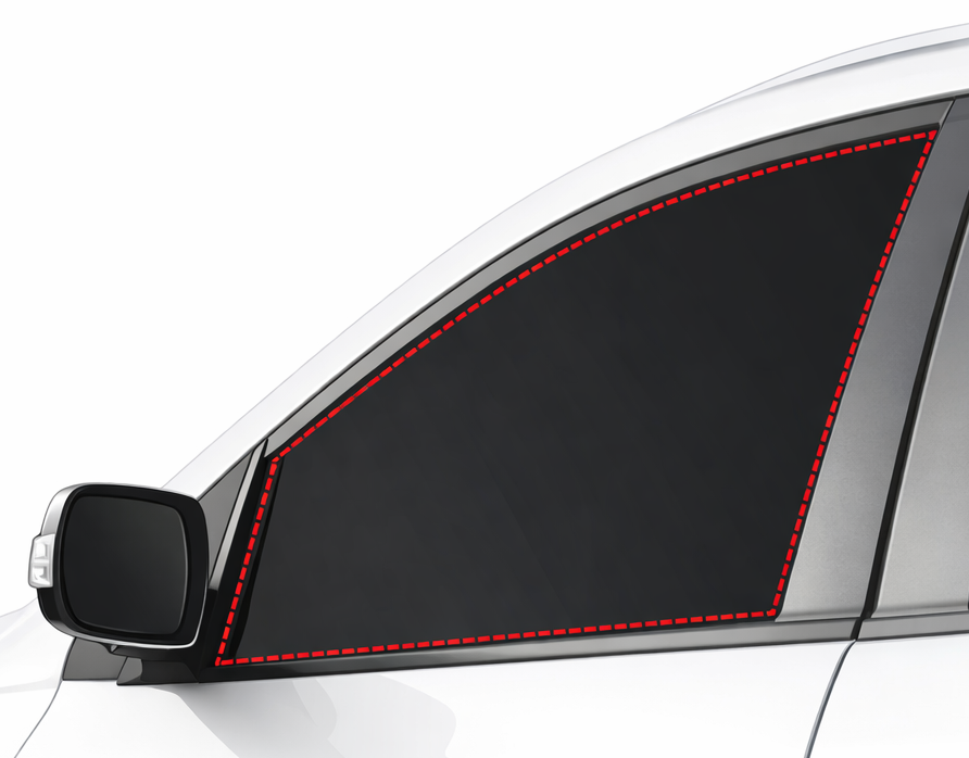
A glass run channel guides and seals a car’s moving window. In the case studied by Nugraha and colleagues, some design values are fixed and the remaining values must be selected to meet performance requirements. The task is to complete the design while preserving those fixed values. Case-study paper.
Forward Prediction and Inverse Design
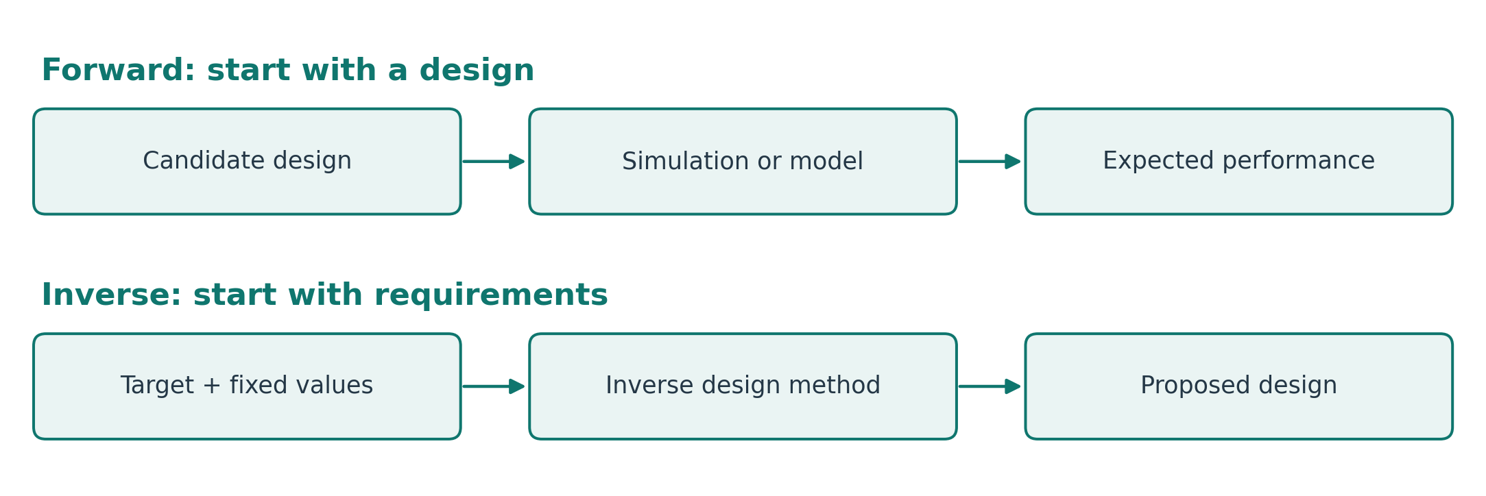
Forward prediction starts with a design and estimates its performance. Inverse design starts with desired performance and seeks a design that could achieve it. This does not mean that a forward model can simply be run backward. Several designs may produce similar performance, and some targets may be impossible under the given constraints.
An inverse method produces candidates. Further simulation or physical testing is needed to assess whether a candidate satisfies the real requirements. The distinction between a predicted result and a verified result is central to engineering applications.
Partial Inverse Design
Partial inverse design chooses only the free design variables while preserving the fixed ones. As a teaching example, suppose dimension A is fixed, dimensions B and C are open, and a target performance is specified. The method proposes B and C, then the complete design is evaluated. These letters are illustrative placeholders, not the paper’s variable names.
The study treats the free design entries as missing values to be estimated. Imputation means estimating missing values from available information. Here the missing entries represent choices to be made, rather than measurements that were lost. Method source.
The Approach: Two Cooperating Networks
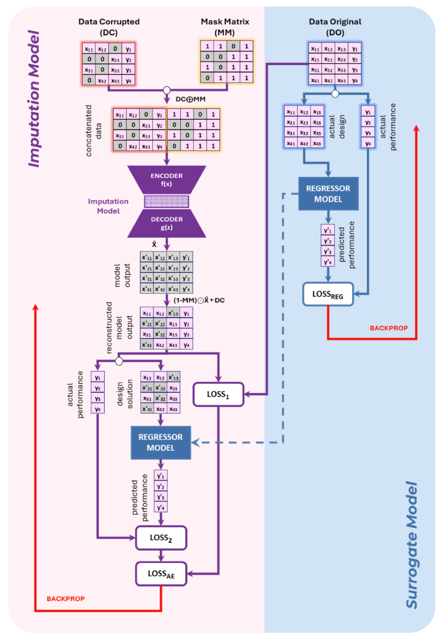
Original manuscript figure from Nugraha et al. (2025).
The study combines an imputation model, which proposes missing values, with a surrogate model, which estimates performance in place of an expensive simulation. Joint training uses reconstruction and performance errors to guide the models. Method source.
Read the original architecture in two parts. On the left, a mask identifies missing entries, and an encoder and decoder reconstruct the design. On the right, the surrogate learns to predict performance from complete designs. The loss terms connect reconstruction and performance during joint training. The red arrows show backpropagation, the process used to update model parameters. The main point for this overview is the role of each model; you do not need to follow every symbol. A surrogate remains an approximation, so agreement with its prediction is not proof of physical validity.
Engineering Case: Results and Limits
The paper reports MSE reductions of up to 98% relative to compared methods and R-squared values of 0.997–0.999 in its initial tests. Reported results.
Mean squared error (MSE) averages squared differences between estimates and reference values; lower values indicate smaller errors. R-squared compares squared prediction error with a reference that predicts the evaluation-set mean. A value closer to 1 indicates a better fit; values can be negative if the model performs worse than that reference. It is not a percentage of correct designs.
“Up to 98%” identifies the largest reported reduction, not the improvement in every experiment. These numbers also do not measure a 98% reduction in cost or design time. The potential application is to help engineers select promising candidates for further validation. New design conditions still require evidence of reliable performance.
3b. Case Study: Well-Log Reconstruction
The Problem: Missing Well-Log Measurements
A well log records measurements along a drilled well’s depth. Logging may take place during or after drilling, and operational or tool problems can leave missing or unreliable values.
Antariksa and colleagues studied missing Vp, or compressional-wave velocity, in the West Natuna Basin, Indonesia. Other available logs supply the inputs; the output is estimated Vp at the required depths. The intended use is to support interpretation of reservoir properties. Case-study paper.
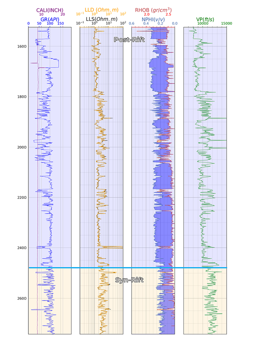
Figure from Antariksa et al. (2023). Read it as a set of measurements arranged along depth; it is not a prediction-versus-reference comparison.
Why Use a Sequence Model?
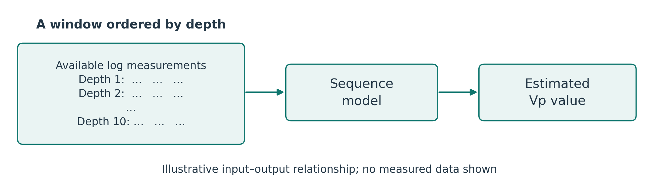
A sequence model learns from observations with a meaningful order. Neighboring depths may provide useful context, although abrupt changes at rock-layer boundaries mean that smoothness cannot be assumed.
The study compared long short-term memory (LSTM), gated recurrent unit (GRU), and bidirectional LSTM models using windows of 10 steps. These are neural-network designs for sequences; bidirectional LSTM processes a sequence in both directions. Here the order is depth, not time. Method source.
Well-Log Case: Results and Limits
LSTM was the best reported model, with MAPE about 2.2% and R-squared about 0.94. The reconstructed logs were used in petrophysical analysis, which interprets rock and fluid properties from measurements. Reported results.
Mean absolute percentage error (MAPE) takes each absolute error as a percentage of its reference value and averages those percentages. An average of 2.2% does not mean every estimate is within 2.2%. MAPE also becomes unreliable when reference values are zero or very close to zero.
An error measure needs known reference values, so evaluation uses available measurements withheld from training. The true values in a genuinely missing interval cannot be compared directly. Domain checks and tests on new wells or geological settings are therefore needed before assuming the same performance elsewhere. Reconstructed values remain estimates.
Glossary
| Term | Meaning |
|---|---|
| Artificial intelligence (AI) | The field of building systems for tasks associated with intelligent behavior |
| Applied AI | The use of AI methods to address practical problems |
| Machine learning (ML) | AI methods in which models learn patterns from data |
| Deep learning | ML methods that use neural networks with multiple layers |
| Model | In this lecture, a learned relationship between inputs and outputs |
| Supervised learning | Learning from examples with known target values or categories |
| Training | Learning or updating a model from data |
| Inference | Applying a trained model to an input |
| Feature | An input variable used by a model |
| Label | The known target value or category in supervised learning |
| Regression | Predicting a numerical value |
| Classification | Assigning an input to a category |
| Forecasting | Predicting future values |
| Anomaly detection | Identifying patterns that differ from expected behavior |
| Generation | Producing candidate outputs, such as designs or text |
| Optimization | Searching for the best feasible option according to an objective |
| Structured data | Data organized into defined fields |
| Unstructured data | Content without a fixed tabular form, such as images or free text |
| Sequential data | Observations with a meaningful order |
| Baseline | A reference method used to judge improvement |
| Validation data | Data used for model selection and adjustment |
| Test data | Data reserved for final evaluation |
| Data leakage | Use of information outside the valid training or prediction setting |
| Deployment | Putting a model into its intended workflow |
| Monitoring | Checking a system’s data, outputs, and performance during use |
| Drift | A change in the data distribution or the relationship between inputs and outcomes |
| Inverse design | Seeking a design from desired performance and requirements |
| Partial inverse design | Choosing free design values while preserving fixed values |
| Imputation | Estimating missing values from available information |
| Surrogate model | A model used as a fast approximation of a more expensive evaluation |
| Sequence model | A model that learns from ordered observations |
| Well log | Measurements recorded along a drilled well’s depth |
| Vp | Compressional-wave velocity |
| Petrophysical analysis | Interpretation of rock and fluid properties using measurements |
| MSE | Mean squared error; the average squared difference from reference values |
| MAPE | Mean absolute percentage error; the average absolute error relative to reference values, expressed as a percentage |
| R-squared | A comparison of squared prediction error with a reference that predicts the evaluation-set mean |
References
- A. Nugraha, H. Kwon, G. Park, and J. Lee (2025). Cooperative neural networks for inverse design: Integrating denoising autoencoder and surrogate model for partial design variable imputation. Engineering Applications of Artificial Intelligence, 162, 112453.
- G. Antariksa, R. Muammar, A. Nugraha, and J. Lee (2023). Deep sequence model-based approach to well log data imputation and petrophysical analysis: A case study on the West Natuna Basin, Indonesia. Journal of Applied Geophysics, 218, 105213.
Return to the Week 1 materials.