Lecture 2 Notes: ML Strategy, Error Analysis, and Simple ML Serving

Note

These notes go with the Lecture 2 slides. They tell the same story in plain words, so you can read them before class to prepare, or after class to review. You do not need any math to follow along. Every new term is explained in simple words where it first appears, and a glossary with formal definitions is at the end.

1. Why do we need ML strategy?

Imagine you built a cat classifier and it reaches 90% accuracy. Not bad, but not good enough. What do you do next?

Collect more data? Train longer? Try a bigger network? A smaller one? Add regularization? Change the architecture? (If some of these words are new to you, do not worry. You will meet all of them during the course.) Every one of these ideas sounds reasonable. That is exactly the problem. Each idea can cost you weeks, and most of them will not help, because they fix problems your model does not have.

Here is the uncomfortable truth: in real projects, the hard part is not training a model. The hard part is deciding what to work on next. Teams without a strategy try things almost at random and can lose months. Teams with a strategy first measure, then diagnose, and only then act.

Think of a doctor. A good doctor does not hand you every medicine in the pharmacy. They diagnose first, then treat. This whole lecture is about how to diagnose a machine learning system.

2. Orthogonalization: one knob, one job

Orthogonalization sounds scary, but it is just a fancy word for a simple idea: each control should do exactly one thing. That is all.

Old TV sets were easy to tune because every knob did exactly one thing: one for brightness, one for contrast, one for position. Now imagine a single knob that changes all three at once. Tuning would be a nightmare.

The same idea applies to ML projects. For a system to work in the real world, four things have to be true, in this order:

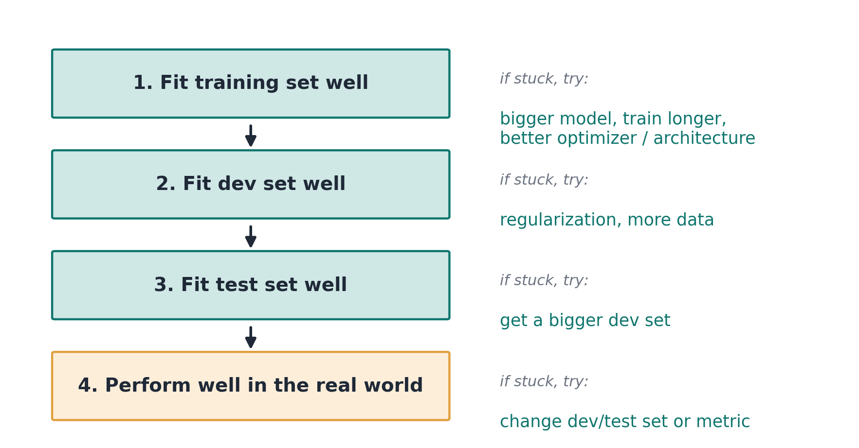
Each stage has its own “knobs”. If your model cannot even fit the training set, more training data will not save you. If it fits training data but fails on new data, a bigger model is probably the wrong knob. Knowing which stage is broken tells you which knobs are even worth touching.

This is why experienced practitioners look calm. When something goes wrong, they know where to look.

3. Pick one number and let it decide

Applied ML is a loop: you get an idea, you code it, you run an experiment, and then you decide whether to keep the change. The faster you go around this loop, the faster you make progress.

The thing that slows teams down most is not coding. It is deciding. Compare these two classifiers:

Classifier	Precision	Recall
A	95%	90%
B	98%	85%

(Quick reminder: precision asks “of everything the model called a cat, how many really were cats?” and recall asks “of all the real cats out there, how many did the model find?”)

Which one is better? You can argue either way, and that argument costs time. Now combine both numbers into one, for example the F1 score (a balanced mix of precision and recall). A scores 92.4%, B scores 91.0%. Done. A wins, next experiment.

One clear number makes every decision instant.

Of course, some numbers should not be maximized. Nobody needs a model that is 1% more accurate but ten times slower. The trick is to split your metrics into two kinds:

Optimizing metric: the one number you want as high as possible.
Satisficing metrics: numbers that only need to be “good enough”, like running time under 100 ms, or memory under some limit.

So instead of arguing about accuracy versus speed, you say: “maximize accuracy, subject to running time below 100 ms.” With N metrics, pick 1 to optimize and turn the other N-1 into simple thresholds. And write your metric down before you start experimenting, not after.

4. Train, dev, and test sets: aim at the right target

Quick reminder of what each set is for:

Set	Job	How often you touch it
Training set	Fit the model	Constantly
Dev set	Compare models, tune choices	Frequently
Test set	Final honest score	Once, at the very end

The dev set (also called validation set) deserves special respect. It is the target you aim at for weeks or months. Every tuning decision pushes your model closer to whatever the dev set contains. So point it at the right thing.

A classic mistake: build the dev set from data of some regions and the test set from data of other regions. The team tunes for months, then discovers they were aiming at the wrong target the whole time. The fix is simple: shuffle everything together first, so dev and test come from the same distribution. (A distribution simply means “the kind of data”: where it comes from and what it typically looks like. Blurry phone photos and sharp studio photos are two different distributions.)

The golden rule, worth memorizing:

Important

Choose dev and test sets that reflect the data you expect to get in the future and consider important to do well on.

About sizes: the old 60/20/20 split made sense when datasets were small. With a million examples, 98/1/1 is fine, because 1% is still ten thousand examples. Do not follow percentages blindly. The dev set just needs to be big enough to tell two models apart, and the test set big enough to give you confidence in the final number.

5. When your metric lies to you

Sometimes the metric and the dev set say one thing and reality says another. Two examples from the lecture:

Algorithm A has 3% error but occasionally shows users inappropriate images. Algorithm B has 5% error and never does. The metric prefers A. You, your users, and your company prefer B. The metric is counting the wrong thing.
Your model scores beautifully on the clean, sharp photos in your dev set, then fails on the blurry phone photos your real users upload. The dev set contains the wrong data.

The rule: if doing well on your metric and dev set does not mean doing well in the real application, do not keep optimizing. Change the metric or change the dev set. A target is only useful if hitting it means winning.

6. Comparing with humans: bias and variance

Why do we compare models with human performance? Because humans are very good at many tasks, and as long as your model is worse than a human, you have tools: humans can label more data for you, and you can ask “why did a person get this example right when the model got it wrong?”

There is also a deeper reason. Some error is simply impossible to remove. Some images are so blurry that nobody, human or machine, can classify them. That unavoidable minimum is called Bayes error. We can never measure it exactly, but for tasks humans do well, the best human performance is a good stand-in for it. Which humans? Take the best you can get: in the medical imaging example from the slides, a typical person scores 3% error, a doctor 1%, an experienced doctor 0.7%, and a team of experienced doctors 0.5%, so 0.5% is our proxy for Bayes error. One more thing to expect: progress feels fast while your model is below human level and the human tools still work, and it usually slows down a lot once you pass it.

This gives us a wonderfully simple diagnosis tool. You need three numbers you already have: human-level error, training error, and dev error. Then look at the two gaps:

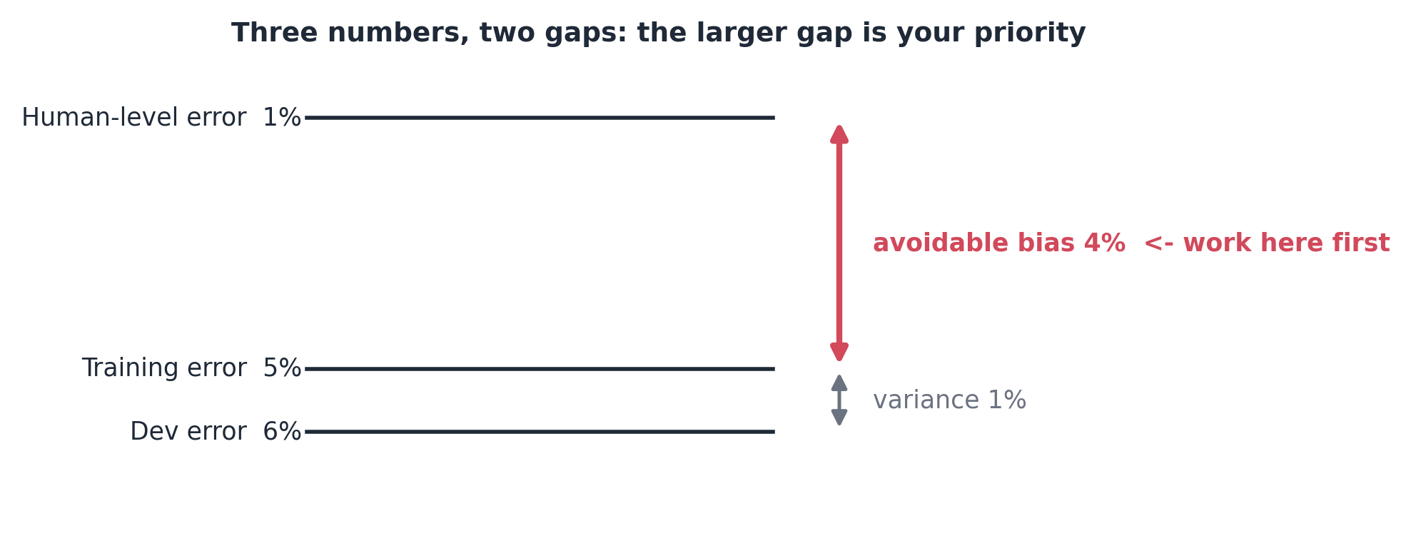
The gap between human level and training error is avoidable bias: the model is not even fitting the training data as well as it could.
The gap between training and dev error is variance: the model memorized the training data more than it learned from it.

Whichever gap is bigger is your priority. And here is the beautiful part: the same numbers can mean opposite things. Training error 8%, dev error 10%. If humans score 1%, you have a big bias problem: work on fitting better. If humans score 7.5% (say the images are genuinely hard), your model is almost as good as possible on training data, so the bias is tiny and the variance gap is what matters.

Once you know the diagnosis, the treatment follows:

Diagnosis	What to try
High avoidable bias	Bigger model, train longer, better optimizer, better architecture
High variance	More data, regularization, data augmentation, simpler model

Notice the tension: a bigger model fights bias but can increase variance, and more data fights variance but does nothing for bias. That is exactly why you diagnose before you treat. “Just collect more data” is only good advice half of the time.

7. Error analysis: just look at your errors

This is the least glamorous and most useful technique in the whole lecture.

Say your cat classifier has 10% error, and a teammate says “it keeps mistaking dogs for cats, let’s spend a month on dog handling.” Before anybody spends a month, spend two hours instead:

Take about 100 misclassified dev set examples.
Look at them, one by one, with your own eyes.
Count what you see.

If only 5 out of 100 errors are dogs, then even a perfect dog fix takes you from 10% to 9.5% error. That is the ceiling of the idea, and it is not worth a month. If 50 out of 100 are dogs, the ceiling is 10% to 5%. Now the idea is exciting.

In practice you check several categories at once in a small spreadsheet: dogs, big cats like lions, blurry images, wrong labels, and whatever else you notice along the way. The category totals tell you where the ceiling is highest:

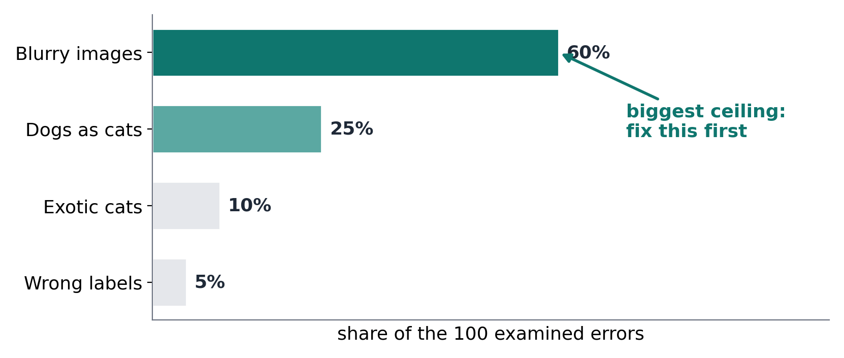
Counting is not a rigid formula, but it turns “I feel like we should fix X” into “fixing X can help at most this much.” Arguments end quickly when the table is on the screen.

A note on wrong labels. In the training set, a few percent of random labeling mistakes are usually harmless; deep learning averages them out. But watch out for systematic mistakes (if white dogs are consistently labeled “cat”, the model will happily learn that rule). In the dev and test sets the question is different: can you still trust your comparisons between models? If bad labels make up a big share of the remaining error, clean them, and clean dev and test the same way so they stay comparable.

8. Build first, then iterate

A tempting trap: spending months designing the perfect system before training anything. Speech recognition has noisy backgrounds, accents, far-away microphones, children’s voices… which one should the architecture handle best? Honest answer: you cannot know in advance.

So do not try to know it in advance. Set up your dev set and metric, build a simple first system quickly, and let its errors tell you what matters.

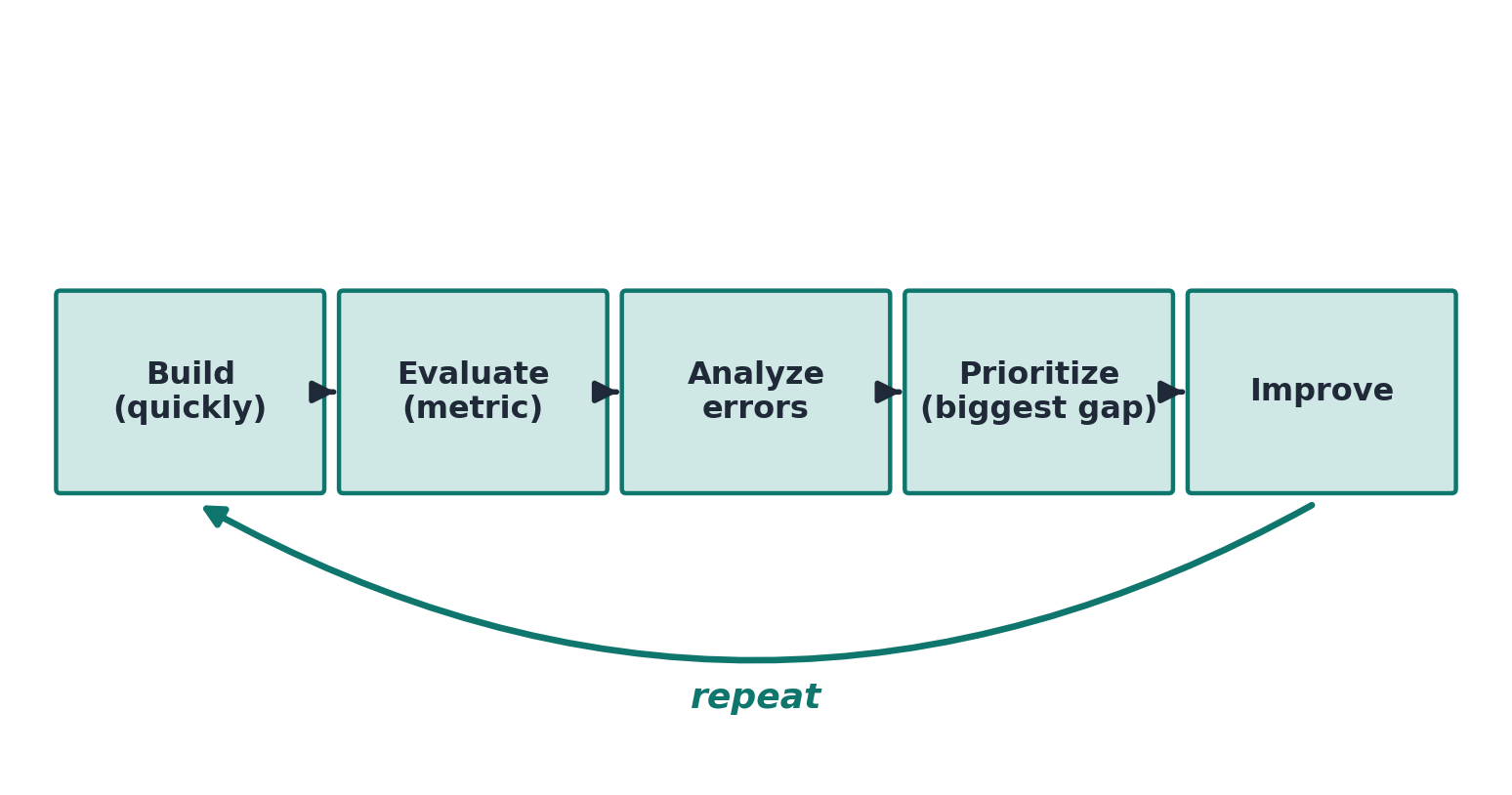
The first system’s job is not to be good. Its job is to generate errors you can study. A working baseline in week one beats a perfect design that is still a diagram in month three. This loop is also exactly how we recommend you run your semester project.

9. When training data and real data are different

In practice, the data you can get and the data you care about are often not the same. You can scrape 200,000 clean cat photos from the web, but your users will upload 10,000 blurry phone photos. Which data goes where?

Resist the urge to shuffle everything together. If you do, your dev set becomes about 95% web photos and you are aiming at the wrong target again. The better split puts the real user data where it counts: dev and test are 100% phone photos, and the training set takes the web photos plus whatever real data is left over.

But now the training set and the dev set come from different distributions, and that breaks our variance diagnosis. If training error is 1% and dev error is 10%, is the model failing to generalize, or is the dev data just harder? Two different problems, two different treatments.

To separate them, carve out a training-dev set: a slice of training-like data that the model never trained on. Now you have four numbers and three gaps:

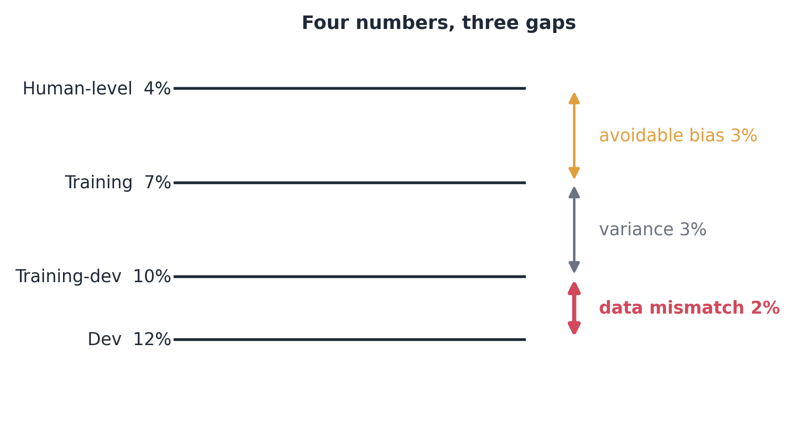
Human level to training error: avoidable bias, as before.
Training to training-dev: variance (same kind of data, only new).
Training-dev to dev: data mismatch (the data itself changed).

If mismatch is your problem, the honest tools are: do manual error analysis to understand exactly how the real data differs (noise? blur? different vocabulary?), make the training data more similar to it, or collect more real data. You can also synthesize data, for example mixing clean speech with car noise to fake in-car recordings. Synthesis works, but be careful: if you repeat one hour of car noise ten thousand times, it sounds fine to you, and the model quietly overfits to that one hour.

10. From model to application: simple ML serving

A trained model sitting in your notebook helps nobody but you. It becomes useful the moment other people and other programs can send it inputs and get predictions back. That step is called serving.

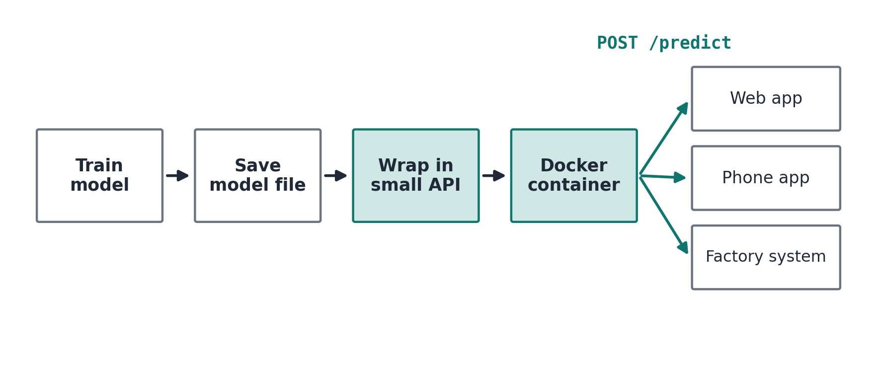
The whole workflow is shorter than it sounds:

Train the model.
Save it to a file.
Wrap it in a small API: one “door” other programs can knock on, like POST /predict, where they send features and receive a prediction. With FastAPI this is about ten lines of Python.
Put the API in a Docker container.
Run the container.
Anyone who can reach the machine can now use your model: a web app, a phone app, a factory system. None of them need Python or your libraries.

And what is Docker? It solves the oldest problem in software: “it works on my machine.” Docker packages your code together with its entire environment (the Python version, the libraries, everything) into one shippable unit.

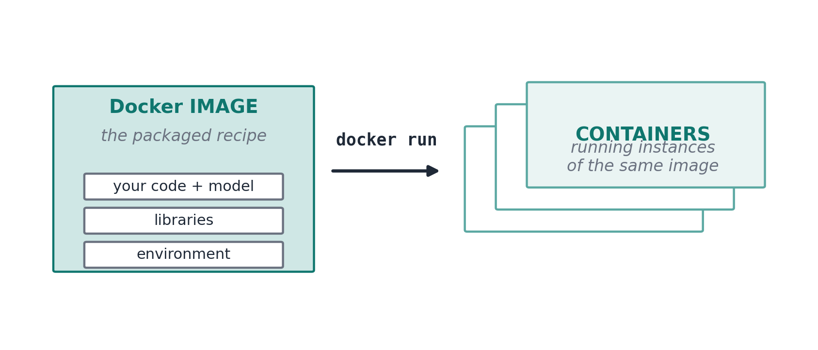
Two words to remember: the image is the packaged recipe, frozen and shareable. A container is that recipe running. You can start many containers from one image, and they behave the same on your laptop, a server, or the cloud. Running one takes two commands:

docker build -t ml-api .
docker run -p 8000:8000 ml-api

You do not need to master Docker in this course. You only need the idea: model, then API, then container, then anyone can use it. We will do this hands-on in the practical weeks.

Key takeaways

Good ML work needs strategy, not random trial and error.
Pick one clear metric, and a dev/test set that looks like the real future data. If they stop reflecting what you care about, change them.
Diagnose before treating: avoidable bias, variance, data mismatch. Three or four error numbers and their gaps tell you what to fix.
Error analysis: look at about 100 errors by hand and count. Fix the category with the biggest ceiling first.
Build a simple system first, then iterate: Build, Evaluate, Analyze, Prioritize, Improve.
A model becomes useful when it is served: API plus Docker connect your model to real applications.

Glossary

Formal definitions of the key terms from this lecture, for reference and exam preparation. The friendlier explanations stay in the sections above, where each term first appears.

Term	Definition
ML strategy	A systematic approach to selecting and prioritizing the actions most likely to improve a machine learning system
Orthogonalization	The design principle of separating controls so that each adjustment affects exactly one aspect of system performance
Dev set (validation set)	A dataset, disjoint from the training set, used to compare models and tune design choices during development
Test set	A held-out dataset used once, after development is complete, to obtain an unbiased estimate of final performance
Distribution	The statistical population from which a dataset is drawn, characterizing the type and properties of its examples
Precision	The fraction of positive predictions that are actually correct
Recall	The fraction of actual positive cases that the model correctly identifies
F1 score	The harmonic mean of precision and recall, combining both into a single evaluation metric
Optimizing metric	The single metric that a project seeks to maximize or minimize during model selection
Satisficing metric	A metric that is only required to meet a predefined threshold rather than be optimized
Bayes error	The lowest error rate achievable by any classifier on a given task; the irreducible error
Human-level performance	The error rate achieved by humans on a task, commonly used as an empirical proxy for Bayes error
Avoidable bias	The gap between training error and the Bayes error proxy; the component of bias that can in principle be eliminated
Variance	The gap between training error and dev (or training-dev) error, reflecting a failure to generalize beyond the training data
Regularization	Techniques that constrain a model during training to reduce overfitting, such as L2 penalties or dropout
Data augmentation	Enlarging a training set by applying label-preserving transformations to existing examples
Overfitting	Fitting the training data, including its noise, so closely that performance on unseen data degrades
Error analysis	Manual inspection and categorization of a sample of misclassified examples to estimate the potential impact of candidate improvements
Ceiling	An upper bound on the performance improvement obtainable by fully resolving a given error category
Baseline	An initial, deliberately simple system built to enable measurement and error analysis before further refinement
Training-dev set	A held-out subset drawn from the training distribution, used to distinguish variance from data mismatch
Data mismatch	A discrepancy between the training distribution and the dev/test distribution that degrades performance independently of bias and variance
Data synthesis	Generation of artificial training examples, for example by combining clean speech recordings with separately recorded noise
Serving	Deploying a trained model so that external users and systems can request predictions from it
API	Application Programming Interface: a defined interface through which programs exchange requests and responses, such as an HTTP endpoint like `POST /predict`
Docker image	An immutable package containing an application together with its complete runtime environment
Docker container	A running instance of a Docker image, isolated from the host system

References for this lecture are listed on the Week 2 page.