Lecture 3 Notes: Deep Learning for Structured and Engineering Data
These notes follow the Lecture 3 slides. Use the explanations and worked examples to review the concepts and equations. Practice questions near the end help you apply the ideas, and the glossary provides a quick reference.
This lecture asks three questions: what can a neural network predict, what useful features can it learn from measurements, and how can several sites train a shared model? We first explain how a network makes predictions and learns. We then consider modeling choices for different engineering situations.
1. Engineering data and prediction tasks
Tabular data are organized into rows and columns. A sample is one row, such as a concrete mix tested in a laboratory. An input feature is one variable supplied to the model. The target is the outcome we want it to predict.
In the concrete example, the inputs describe the cement, water, fly ash, curing age, and temperature. The target is the measured compressive strength. During training, the model compares its predictions with those measurements. For a new mix, the inputs are supplied and strength is predicted; the measured strength is not an input.
TABLE. Concrete Inputs and Targets
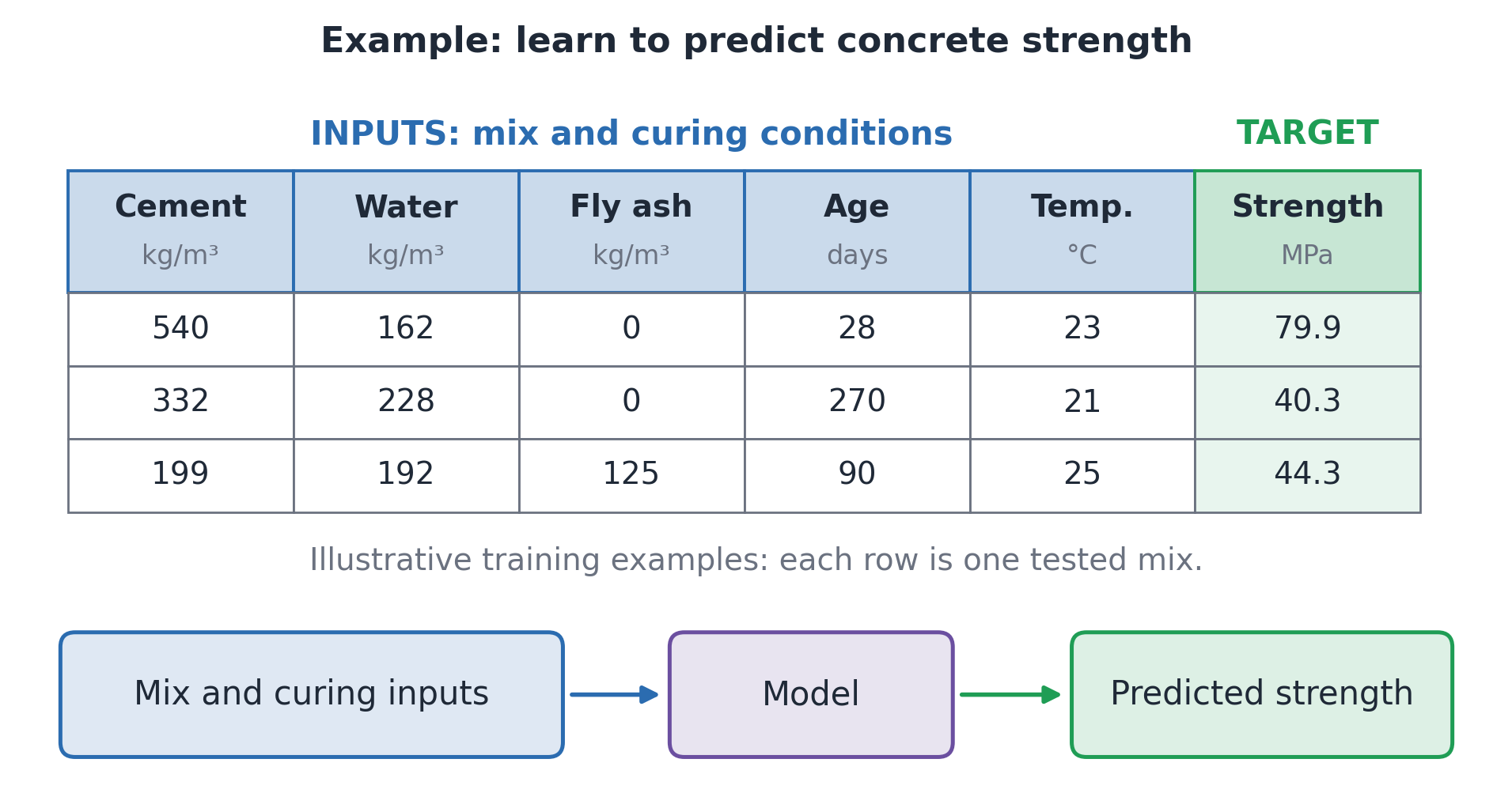
The same input-to-outcome pattern appears in other applications. Material composition may help predict strength; machine sensors may help detect a fault; production settings may help estimate product quality. Predicting a number is regression. Predicting a category, such as healthy or faulty, is classification.
A neural network is not automatically the best choice. A baseline is a comparison model used to judge whether a more complex method is worthwhile. On small tabular datasets, random forests or gradient-boosted models can be strong baselines. Neural networks become useful candidates when learning features from complex measurements or reusing what was learned on another task. The choice should be checked on data representative of the intended use.
2. From linear models to neurons and multilayer perceptrons
A linear model combines inputs with weights and adds a bias:
z=w_1x_1+\cdots+w_nx_n+b.
Each weight controls one input’s contribution to the sum. The bias shifts the sum. An artificial neuron applies an activation function f to produce an output, a=f(z). A nonlinear activation allows a network to represent relationships beyond a linear combination of the original inputs.
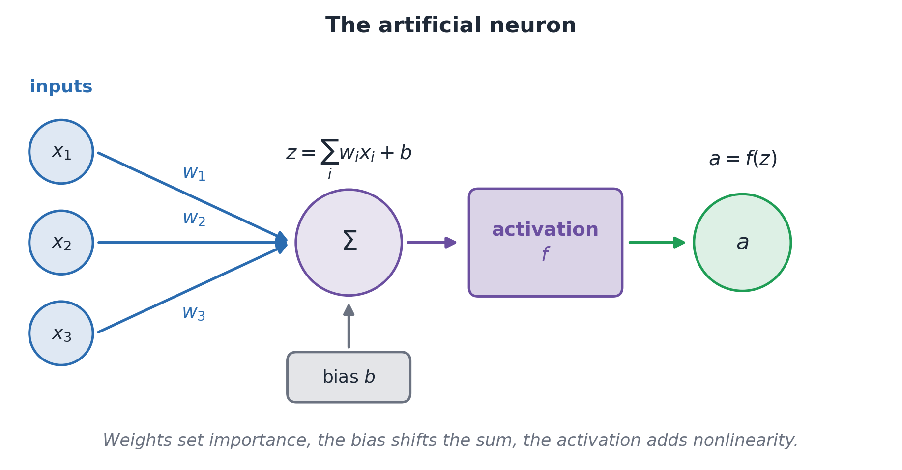
A hidden layer is between the inputs and the final prediction. Its units learn combinations of measurements that help with the task. These learned features form a representation of the input. The engineer chooses the architecture, but training learns the weights. A useful hidden feature need not correspond to a named physical quantity.
A multilayer perceptron (MLP) has fully connected layers: each unit receives the outputs of the previous layer. One layer can be written as h=f(Wx+b), where W contains its weights, b its biases, and h its outputs. The slide’s larger illustrative network takes eight input features, has hidden layers of 64 and 32 units, and produces one numerical prediction. These layer sizes are choices to evaluate, not fixed rules.
Without nonlinear activations, a stack of linear layers is equivalent to one linear layer. With biases, it remains one affine transformation. Common activation choices include:
- ReLU: \max(0,z), often used in hidden layers.
- Sigmoid: maps one score to a value between zero and one, often used for a binary probability.
- Softmax: maps several scores to class probabilities that sum to one.
A numerical prediction often uses no final activation. If the quantity has a physical limit, an appropriate output transformation may be useful.
We write the whole prediction as \hat y=f_\theta(x). Here x is the input, \theta is the collection of weights and biases, and \hat y is the output. Training adjusts \theta to reduce the training loss.
3. How a network learns
The forward pass computes a prediction. A loss function measures its error and gives training an objective: the quantity it aims to reduce. For numerical targets, mean squared error is a common choice.
L=\frac{1}{N}\sum_i(y_i-\hat y_i)^2.
N is the number of examples, y_i the measured target, and \hat y_i the prediction. In the slide’s example, measured strength is 70 MPa and predicted strength is 52 MPa. The error magnitude is 18 MPa, so the squared error for that example is 324 MPa squared. Classification commonly uses cross-entropy loss. Accuracy is useful for reporting classification performance, but its abrupt changes do not provide a useful gradient for ordinary gradient-based training.
A gradient gives the local sensitivity of the loss to the parameters. Backpropagation computes these gradients efficiently by working backward through the network’s calculations. It uses the chain rule, which relates the derivative of a sequence of functions to the derivatives of its parts. Backpropagation does not itself change the parameters. The optimizer uses the gradients to make an update, such as gradient descent:
\theta\leftarrow\theta-\eta\nabla_\theta L.
The learning rate \eta controls the update size. A very small value may make learning slow; a large one may cause unstable training. The gradient gives local information, not the location of the global minimum.
Interpreting the gradient update: \nabla_\theta L collects the loss derivatives with respect to the parameters. For one parameter, a positive slope means a small move to the left reduces the loss locally. Subtracting the gradient implements that direction. The learning rate scales the move.
One update in the strength example: the network predicts 52 MPa for a sample whose target is 70 MPa. Its squared error is 324 MPa squared. Backpropagation computes how the loss changes with the parameters, and the optimizer uses those gradients to update them. The next prediction uses the updated parameters.
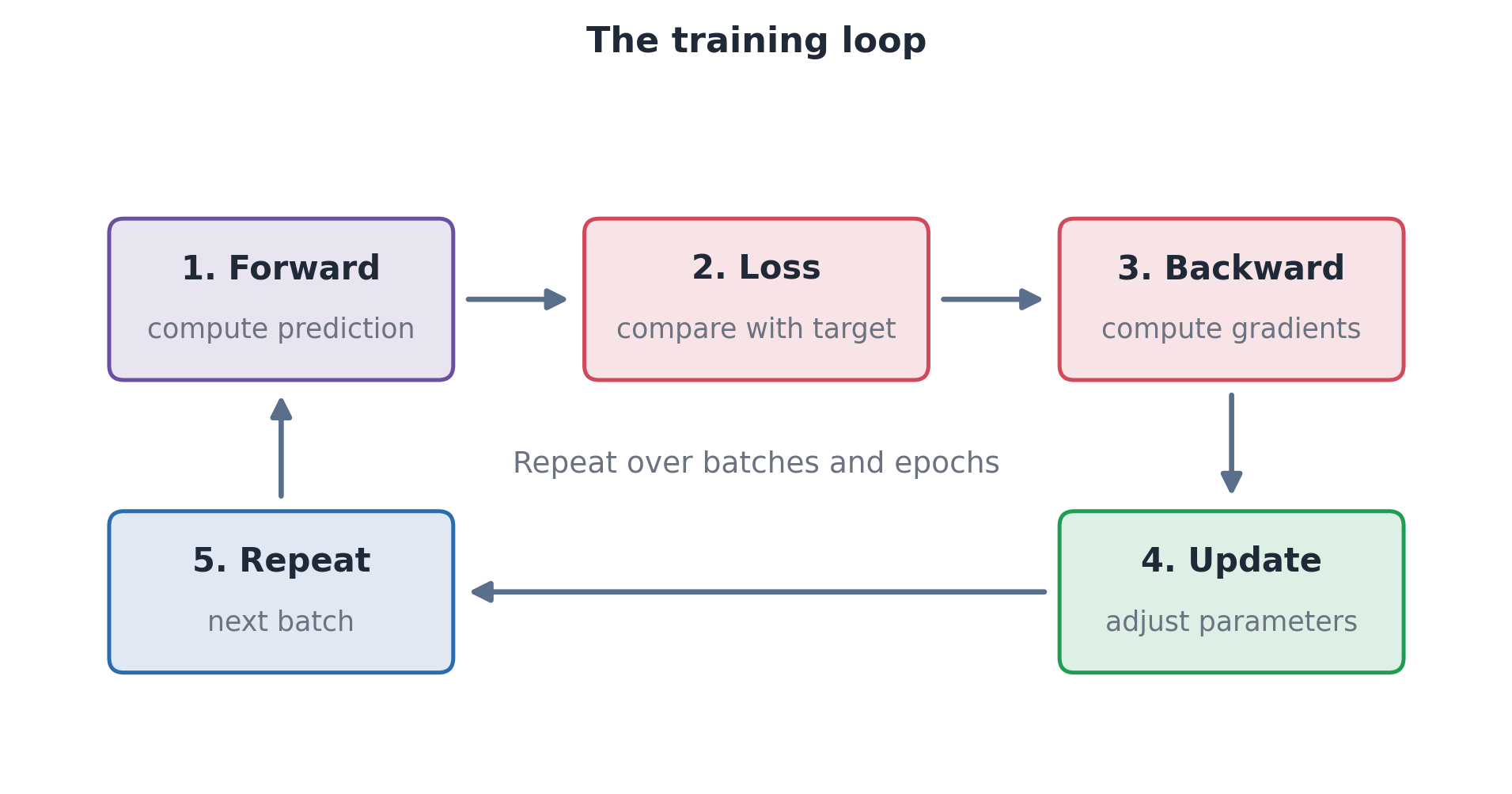
A batch is a group of examples used for one update. An iteration here means one update, and an epoch is one pass through the training set. With 1,000 examples and batches of 100, one epoch has ten updates. Smaller batches give noisier estimates of the full-data gradient. Optimizers include stochastic gradient descent (SGD), SGD with momentum, Adam, and AdamW. Momentum uses a history of updates; Adam adapts updates using running gradient statistics. Optimizer choice still needs validation.
The dataset roles are different:
| Dataset | Purpose |
|---|---|
| Training | Adjust the model parameters |
| Validation | Choose settings and a stopping point |
| Test | Assess the selected model on held-out examples |
Do not tune the model using test results. The split must also reflect the intended use and avoid leakage, such as putting nearly identical observations on both sides of a split.
Overfitting occurs when a model fits the training examples but performs poorly on new examples. Falling training loss with rising validation loss is a warning. Possible responses include better data, a simpler model, and regularization, meaning training choices that discourage fitting accidental details. Weight decay discourages large weights. Dropout removes some activations at random during training. Early stopping keeps a model associated with a better validation result.
4. Neural networks in PyTorch
PyTorch is a Python library that provides the data, model, and gradient tools needed to implement the training loop in code.
The examples connect concepts to recognizable code; they are not a complete standalone training program. Three terms are useful: tensors store numerical data, modules define layers or complete networks, and autograd computes gradients.
A tensor is an array of numbers. This small example has two samples with three features each:
import torch

x = torch.tensor([[0.5, 1.2, 3.1],
                  [0.7, 0.9, 2.8]])

print(x.shape)   # torch.Size([2, 3])
For these tabular inputs, rows are samples and columns are features. The feature count must match the model input. The next example uses a different, eight-feature input. Linear combines inputs using weights and biases, ReLU adds a nonlinear response, and the final layer returns one prediction.
from torch import nn

model = nn.Sequential(
    nn.Linear(8, 64), nn.ReLU(),
    nn.Linear(64, 32), nn.ReLU(),
    nn.Linear(32, 1),
)
Once the model, loss function criterion, and optimizer have been set up, one update has these steps. For this eight-input model, x has shape (batch_size, 8) and y has shape (batch_size, 1) for the corresponding numerical targets:
optimizer.zero_grad()               # clear old gradients
prediction = model(x)               # forward pass
loss = criterion(prediction, y)     # measure the error
loss.backward()                     # compute gradients
optimizer.step()                    # update parameters
backward() computes gradients; step() changes parameters. PyTorch normally accumulates gradients, so previous gradients must be cleared before computing them for this update, unless accumulation is deliberate.
Autograd handles the differentiation needed for training. It tracks the required operations when gradient tracking is enabled and the relevant tensors require gradients. Network parameters normally do; inputs need gradient tracking only when their derivatives are required. Computation may run on a CPU or a supported GPU. Moving the model is not enough: its input tensors, and targets used in the loss, must also be on the appropriate device.
IV) Modern Modeling Paradigms for Engineering AI
The first half used a simple prediction example. The next topics ask different questions about learning features, sharing data or models, and using specialized predictors. A modeling approach describes how we use data and knowledge for a task. These choices can sometimes be combined; they are not levels or compulsory stages.
Choosing an approach: start from the problem’s needs, such as scarce labels or restricted data sharing. Each section shows how a particular choice can address one of those needs.
| Topic | Slides |
|---|---|
| IV) Overview | 27–29 |
| IV.A) Representation learning and self-supervision | 30–34 |
| IV.B) Local, global, and foundation models | 35–39 |
| IV.C) Federated learning | 40–44 |
| IV.D) Mixture of experts | 45–48 |
| IV.E) Comparing and choosing approaches | 49–54 |
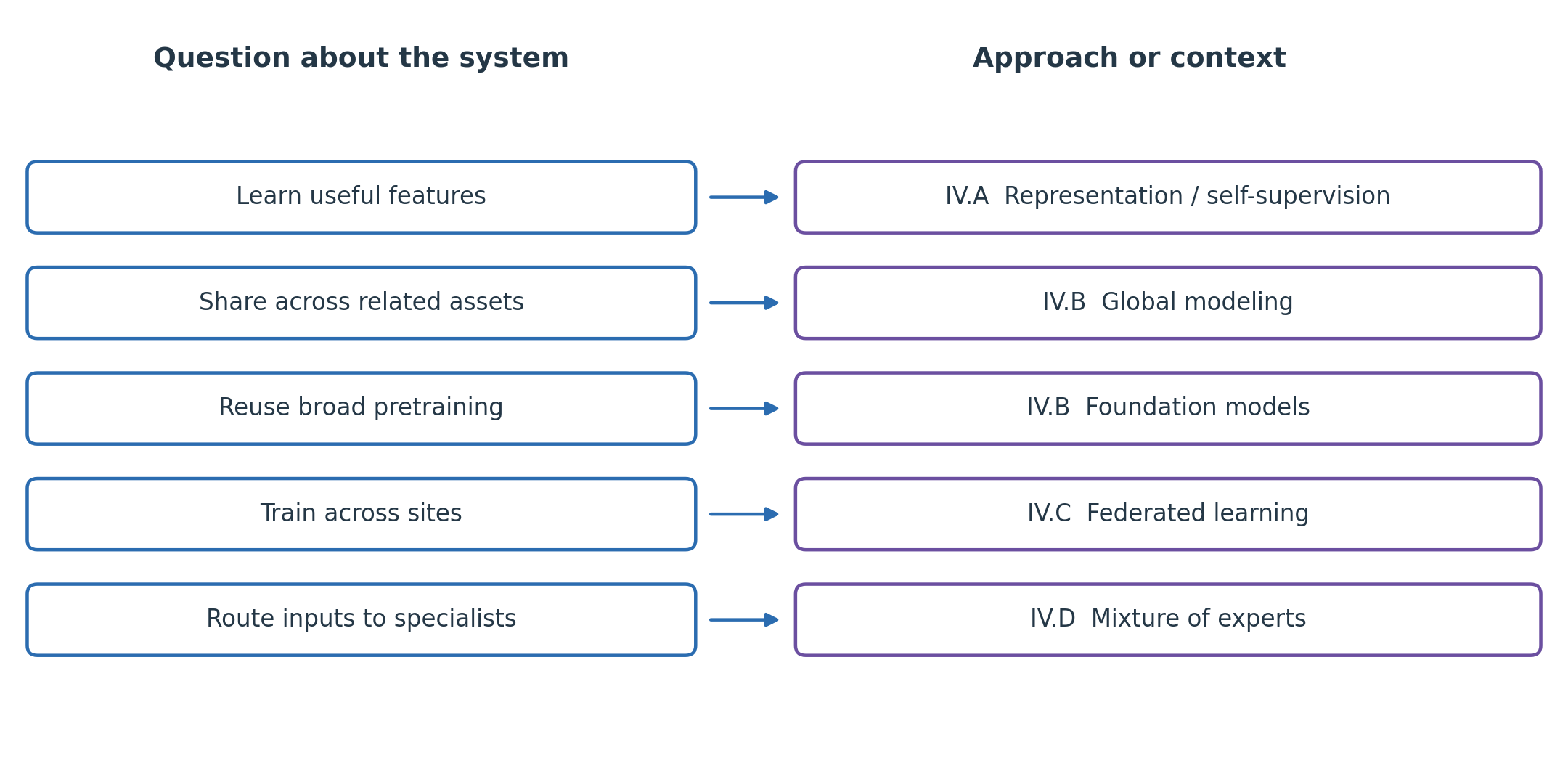
The map separates different questions about a learning system. Global modeling concerns learning across assets; federation concerns where training happens. A shared model can therefore be trained through federated learning. The approaches can be combined when they address different needs.
IV.A) Representation Learning and Self-Supervision
A label is a known target for a task, such as a confirmed bearing failure. A factory may have ten years of vibration recordings but only forty documented failures. The unlabeled recordings may still contain useful patterns. Representation learning learns useful features from data. It can be supervised, but here we are interested in using data without external task labels.
The aim in this example: learn features from the many unlabeled recordings, then use the few fault labels to train a detector. Test whether those features improve fault detection.
Representation learning is the broad idea; an autoencoder is one method. The learned features can support classification, regression, clustering, anomaly detection, or forecasting. Their usefulness depends on the task and must be checked on suitable data.
An autoencoder learns to reconstruct its input. The encoder maps the input x to a learned representation z. The decoder uses z to produce a reconstruction \hat x. Training reduces reconstruction error, for example \lVert x-\hat x\rVert^2, the sum of squared differences between the input and its reconstruction 1.
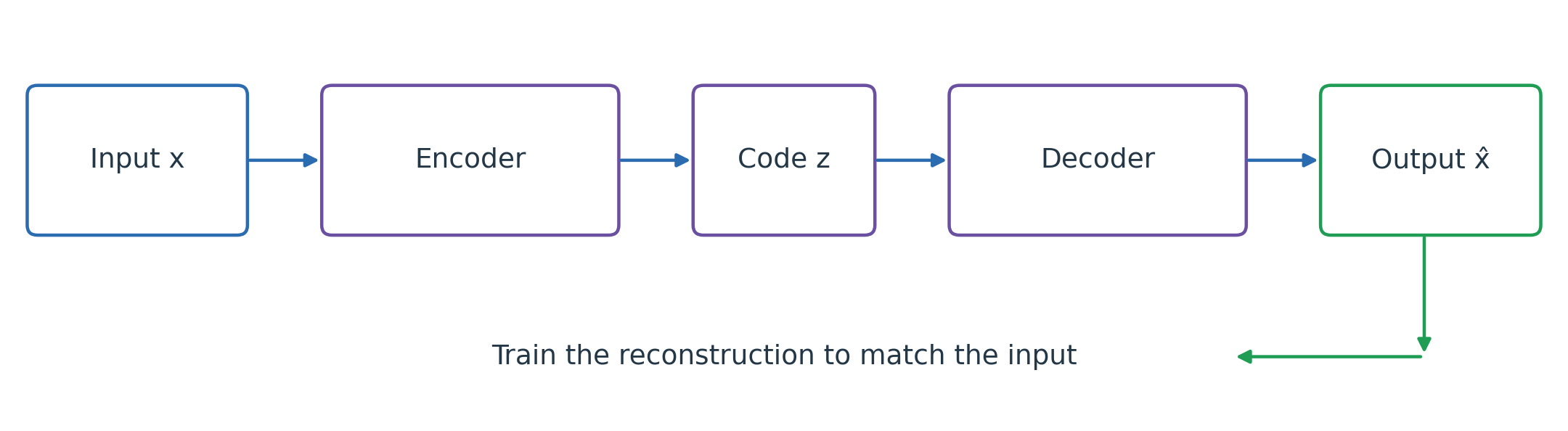
The representation z is often called latent because its variables are learned rather than measured directly. A narrow bottleneck limits the representation’s size, but it does not guarantee useful or physically meaningful features. A model may reconstruct ambient variation well while missing the patterns needed for fault detection. High reconstruction error means the model reconstructed a sample poorly. It can be used to flag possible anomalies, but it does not by itself establish a fault.
Three useful autoencoder variants are:
- A standard autoencoder reconstructs its input.
- A denoising autoencoder reconstructs a clean input from a corrupted version.
- A variational autoencoder (VAE) learns a probabilistic model of the data. Its encoder estimates a distribution of latent codes for each input. Training balances reconstruction with a penalty that keeps these distributions close to a chosen reference distribution, called the prior. To generate a new example, sample a code from the prior and pass it through the decoder 8.
Choosing an autoencoder variant: match the training task to the aim. Reconstructing inputs, removing corruption, and learning to generate samples require different training setups. A more elaborate variant is not automatically better for the intended task.
Self-supervised learning creates its training targets from the data themselves. For example, hide a sensor reading and predict it from the remaining readings. Other objectives reconstruct inputs or learn which views of a sample should be similar. Such an auxiliary objective is often called a pretext task. A downstream task uses the learned representation or pretrained model for a later purpose, such as fault detection or forecasting. Evaluate whether the learned features improve its results.
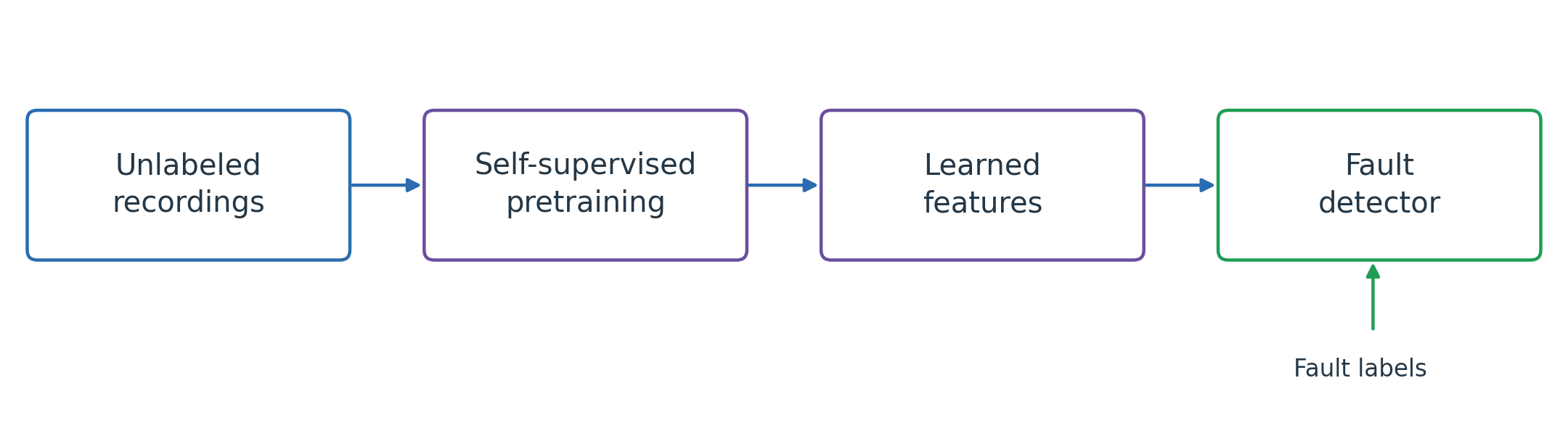
From pretraining to fault detection: pretraining uses the many recordings to learn features. The later fault detector uses those features with the available failure labels. In the masking example, the original hidden reading supplies the training target. Predicting a future region from earlier observations is another possible self-supervised task. These objectives extend beyond the standard autoencoder’s input-reconstruction task.
IV.B) Local, Global, and Foundation Models
Local and global models
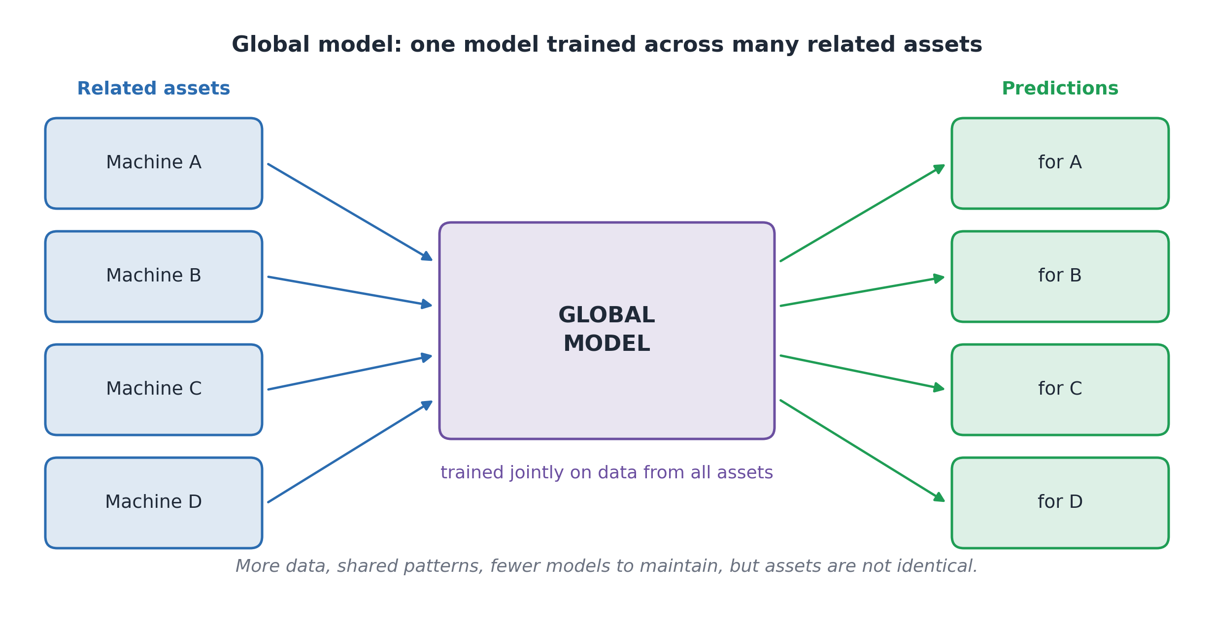
An asset is an individual machine or system, such as one pump. A local model is trained for one asset. A global model learns from several related assets and makes predictions for them 3.
A global model may help when each pump has little history. It may use pump identity or operating conditions as inputs. However, pumps can differ in age, load, and environment. Compare local and global models, and evaluate performance for each asset as well as overall.
Foundation models
A foundation model is trained on broad, diverse data at scale so it can be adapted to many tasks 4. Pretraining is the initial training whose learned parameters will be reused. Adaptation prepares the model for a particular task; fine-tuning does this through further training. Pretraining may use supervised or self-supervised objectives.
For example, a broadly pretrained sensor model might be adapted to forecasting or fault classification. This differs from a global model serving one task across a fleet: global modeling shares learning across assets; foundation models support reuse across tasks. Before adapting a model, check its fit to the new sensors, units, equipment, and operating conditions. Compare it with established methods on the new task.
Training a fault predictor on more pumps does not by itself make it a foundation model. Broad pretraining and adaptability across tasks are the relevant properties, rather than data volume alone.
IV.C) Federated Learning
Federated learning trains a shared model across sites without gathering all the raw training data in one place. Each participating site, or client, trains locally and shares model updates, such as updated parameter values. This may help factories collaborate when production data are confidential or expensive to transfer.
One training round
In the server-coordinated example, the server sends the current shared model to participating clients. They train local copies, return updates, and the server combines them. Each round turns local learning into the next shared model while raw records stay at the clients. FedAvg uses a sample-count-weighted average 5. Consider three clients with the following example counts:
| Client | Training examples | Share of total |
|---|---|---|
| A | 1,000 | 50% |
| B | 500 | 25% |
| C | 500 | 25% |
| Total | 2,000 | 100% |
Divide each client’s count by 2,000. This gives:
w_{\mathrm{global}}=0.50w_A+0.25w_B+0.25w_C.
The general form is:
w_{\text{global}}=\sum_k\frac{n_k}{N}w_k.
w_k contains client k’s parameters after local training, n_k is its training-example count, and N is the total across participating clients. Clients start from the same shared parameters and use the same model structure so corresponding parameters can be averaged. A client with more examples has a larger weight in this version of FedAvg.
Worked parameter example: suppose one corresponding parameter is 2 at A, 4 at B, and 6 at C after local training. Its aggregated value is 0.50(2)+0.25(4)+0.25(6)=3.5. Repeat the operation for each corresponding parameter. This combines learned parameters, not raw records or predictions.
The server’s shared model is often called the global model in federated learning.
Practical challenges
Keeping raw data local does not guarantee privacy because model updates can reveal information about the training data. Communication also takes time, and clients may have different computing resources or may be unavailable for a round.
Different data across clients
The slide uses hypothetical healthy operating temperatures of 50°C, 70°C, and 90°C at three factories. These are not operating limits. Different equipment or conditions can produce different normal temperatures. A fault detector that ignores those conditions could mistake healthy operation at one factory for a fault.
The curves show distributions of readings, not temperature changing over time.
IID means independent and identically distributed samples. The factories have different distributions, so the example illustrates non-IID data. Different local data can produce different model updates, and a shared model may work better at some factories than at others.
Takeaway: good overall accuracy does not establish that the shared model works well at every factory. Evaluate it separately at each site before use. For a fault detector, check both missed faults and false alarms. The healthy 90°C readings at Factory C show why local operating conditions matter.
IV.D) Mixture of Experts
A ship may behave differently during maneuvering, cruising, and heavy weather. These conditions are operating regimes. If a single predictor has systematic errors in some regimes, several specialized predictors may help. First compare with a model that already includes operating conditions as inputs.
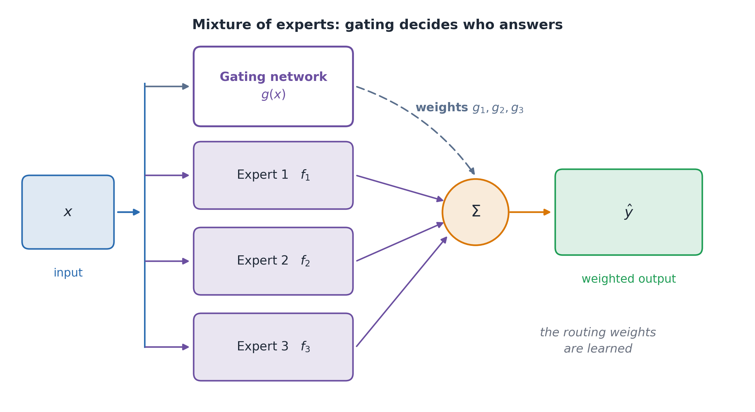
A mixture of experts combines submodels called experts. A gating network learns how much each expert contributes from the input 6.
For the illustrative ship input of 18 knots, 0.5 m waves, and 75% engine load, the gate assigns the following weights to the expert predictions:
| Expert | Gate weight | Predicted fuel use |
|---|---|---|
| 1 | 0.80 | 20 tonnes/day |
| 2 | 0.05 | 30 tonnes/day |
| 3 | 0.15 | 24 tonnes/day |
\hat y=0.80(20)+0.05(30)+0.15(24)=21.1\text{ tonnes/day}.
Interpreting the result: the weighted contributions are 0.80(20)=16, 0.05(30)=1.5, and 0.15(24)=3.6 tonnes/day. Their sum is 21.1 tonnes/day. Expert 1 has the most influence because its weight is 80%. Another operating condition may emphasize different experts. These values are hypothetical predictions, not measured observations.
The general expression is:
\hat y=\sum_i g_i(x)f_i(x).
f_i(x) is expert i’s prediction, and g_i(x) its gate weight. In the mixture shown, weights are nonnegative and sum to one. The gate and experts learn together. Different inputs can use different combinations of predictions.
An ordinary averaging or voting ensemble usually evaluates all its members. A sparse mixture selects only a few experts per input to reduce computation. Mixtures can also be described as ensembles; the comparison concerns the combination rule, not mutually exclusive categories.
Evaluating expert specialization: check whether input-dependent specialization improves predictions enough to justify its extra complexity. Compare with a simpler model and check that the gate uses its experts effectively, rather than leaving some unused. Experts do not automatically learn human-named regimes such as cruising or heavy weather. Check what each expert has learned before assigning it such a physical interpretation.
IV.E) Comparing and Choosing Approaches
A network diagram alone does not explain a modeling approach. Identify the task, training objective, data sources, and intended use. The same type of network may play different roles, and different methods may be combined when the problem justifies it.
| Approach or context | When to consider it | Main idea | What to check |
|---|---|---|---|
| Self-supervised features | Few task labels | Learn from targets created from the inputs | Do the features help the final task? |
| Global model | Many related assets | Share learning across assets | Performance on each asset |
| Foundation model | Several tasks to adapt to | Reuse a broadly pretrained model | Fit to the new data and task |
| Federated learning | Data stay at different sites | Train locally and combine updates | Local performance, privacy, communication |
| Mixture of experts | Different operating conditions | Learn how to combine specialized models | Accuracy, cost, use of each expert |
Practice questions: for each situation below, propose an approach and explain why it may help. Identify a suitable baseline and how you would evaluate the result. More than one approach may be reasonable.
- A. Ten years of vibration data, but only 40 confirmed bearing failures.
- B. Five companies with similar machines cannot share raw production data.
- C. A ship’s fuel use differs during maneuvering, cruising, and heavy weather.
Suggested reasoning: A may benefit from self-supervised features, and B from federated learning. For C, compare expert models with a simpler model that uses operating conditions as inputs. Each choice needs an evaluation plan.
When reading a paper, inspect its inputs, outputs, objective, assumptions, constraints, baseline, and results on unseen cases. A method’s name is not evidence that it solves the intended engineering problem.
Glossary
Use this glossary to review the terms introduced in the lecture. Definitions refer to the examples and training methods used here.
| Term | Definition |
|---|---|
| Neural network | A model built from connected computational units with learnable parameters, organized in layers |
| Multilayer perceptron (MLP) | A feedforward neural network with fully connected layers and nonlinear hidden-layer activations |
| Weight | A learnable coefficient that scales an input to a neuron |
| Bias | A learnable additive term in a neuron’s weighted sum |
| Activation function | A function applied to a neuron’s weighted sum or a layer’s outputs; nonlinear activations let a network learn nonlinear relationships |
| Forward pass | The evaluation of the network from inputs to outputs for the current parameter values |
| Loss function | A numerical measure of prediction error or another training objective that the model aims to minimize |
| Gradient | The vector of partial derivatives of the loss with respect to the parameters, evaluated at the current parameter values |
| Gradient descent | An optimization method that updates parameters in the direction opposite to the gradient, scaled by the learning rate \eta |
| Backpropagation | The algorithm that computes the gradient of the loss with respect to every parameter by applying the chain rule backward through the computational graph |
| Epoch | One complete pass of the training algorithm over the entire training set |
| Batch (mini-batch) | The subset of training samples used to compute one gradient estimate and one parameter update |
| Iteration | A single parameter update, computed from one batch |
| Learning rate | A factor that scales parameter updates; the update also depends on the gradients and the optimizer |
| Optimizer | The rule that converts gradients into parameter updates, such as SGD, SGD with momentum, Adam, or AdamW |
| Training set | The data used to fit the model parameters |
| Validation set | Held-out data used to select the architecture, hyperparameters, and stopping point |
| Test set | Held-out data used for final assessment, never used to tune choices |
| Overfitting | Learning training-specific patterns, including noise, that do not generalize well to new data |
| Dropout | A regularization method that randomly disables a subset of units on each training pass, discouraging reliance on particular activations |
| Tensor | In the array programming used here, an array of numbers with zero or more dimensions; scalars, vectors, and matrices are examples |
| Autograd | PyTorch’s automatic differentiation system, which tracks operations and computes derivatives such as the gradients needed for training |
| Modeling paradigm | An approach to organizing how a model learns and is used, including its objective, data sources, and prior knowledge |
| Representation learning | Learning features from data through a training objective, rather than specifying all features by hand |
| Latent representation | An internal description of an input in terms of variables that are not directly observed, such as the code z in an autoencoder |
| Latent space | The set of possible latent representations; the training objective influences how they are organized |
| Encoder | A component that maps an input to a representation; in a VAE, it specifies a distribution over latent codes |
| Decoder | A component that maps a latent representation to an output, such as an autoencoder’s reconstruction |
| Autoencoder | A neural network trained to reconstruct its input through an encoder and decoder, using the input as its reconstruction target |
| Bottleneck | A restriction on a representation, often a smaller number of latent variables, intended to encourage a compact encoding |
| Reconstruction error | A measure of difference between an input and its reconstruction, such as the squared error \lVert x-\hat{x}\rVert^2 used here |
| Denoising autoencoder (DAE) | An autoencoder trained to reconstruct a clean input from a corrupted version of that input |
| Variational autoencoder (VAE) | A probabilistic generative model with an encoder that estimates latent-code distributions and a decoder that models the data; training balances reconstruction and regularization toward a prior distribution |
| Self-supervised learning | Learning with training targets or supervisory signals constructed from the data themselves |
| Pretext task | A training task used to learn representations for later use, such as predicting a deliberately hidden sensor reading |
| Downstream task | A later task that uses a pretrained model or learned representation, such as fault detection or forecasting |
| Local model | In the multi-asset setting here, a separate model fitted to an individual asset’s data |
| Global model | In the multi-asset setting here, one model fitted using data from multiple assets; in federated learning, the term also names the shared model maintained across clients |
| Foundation model | A model trained on broad data at scale that can be adapted to a wide range of downstream tasks |
| Pretraining | Initial training whose learned parameters are reused or adapted for a later task; it may use supervised or self-supervised objectives |
| Fine-tuning | Further training that updates some or all of a pretrained model’s parameters for a target task or dataset |
| Federated learning | Collaborative model training in which participants keep their training data locally and exchange model information, such as parameter updates |
| FedAvg | The basic federated aggregation rule w_{\text{global}} = \sum_k (n_k/N) w_k, which averages client parameters weighted by each client’s number of local samples |
| Client | A participant in federated learning, such as a factory or device, that holds local data and can perform local training |
| Aggregation | Combining client updates into an updated shared model, for example by averaging parameters in FedAvg |
| IID | Independent and identically distributed: samples are independent draws from the same distribution |
| Non-IID | Data that do not satisfy independence, identical distribution, or both; the lecture’s factory example has different distributions across clients |
| Mixture of experts | A model containing several specialized expert submodels together with a gating mechanism that determines which expert or combination of experts processes each input |
| Expert | A submodel in a mixture of experts whose output contributes according to the gate’s selection or weights |
| Gating network | The component that maps an input to routing weights g_i(x) over the experts, learned jointly with the experts |
| Sparse mixture of experts | A mixture in which the gate selects only a subset of experts to process each input |
References for this lecture are listed on the Week 3 page.