Lecture 4 Notes: Time-Series Forecasting and Anomaly Detection
These notes follow the Lecture 4 slides, using the same section codes, examples, and calculations. Read the explanations alongside the figures, and try each practice question before opening its answer. The full reference list is on the Week 4 page.
Machine temperature, vibration, electricity demand, and traffic all change over time. This lecture connects two questions:
- Forecasting: what do we expect to happen next?
- Anomaly detection: is what actually happened consistent with the behavior we expect?
Both require an appropriate expectation. A forecast may use recent sensor history and operating conditions. A detector may compare a new reading with that forecast, a trusted healthy period, or an engineering limit. A useful result must also support a decision, such as planning demand or investigating a machine.
The main examples use machine temperature and RPM, meaning revolutions per minute. All plotted data, numerical examples, and thresholds are hypothetical. They illustrate the methods and are not equipment operating limits.
I.A) Understanding Time-Series Data
Reading a time-series graph
A time series is a sequence of observations recorded over time. In the graph below, each point is an hourly temperature reading from one machine. The horizontal axis shows when a reading was taken; the vertical axis shows its value in degrees Celsius.
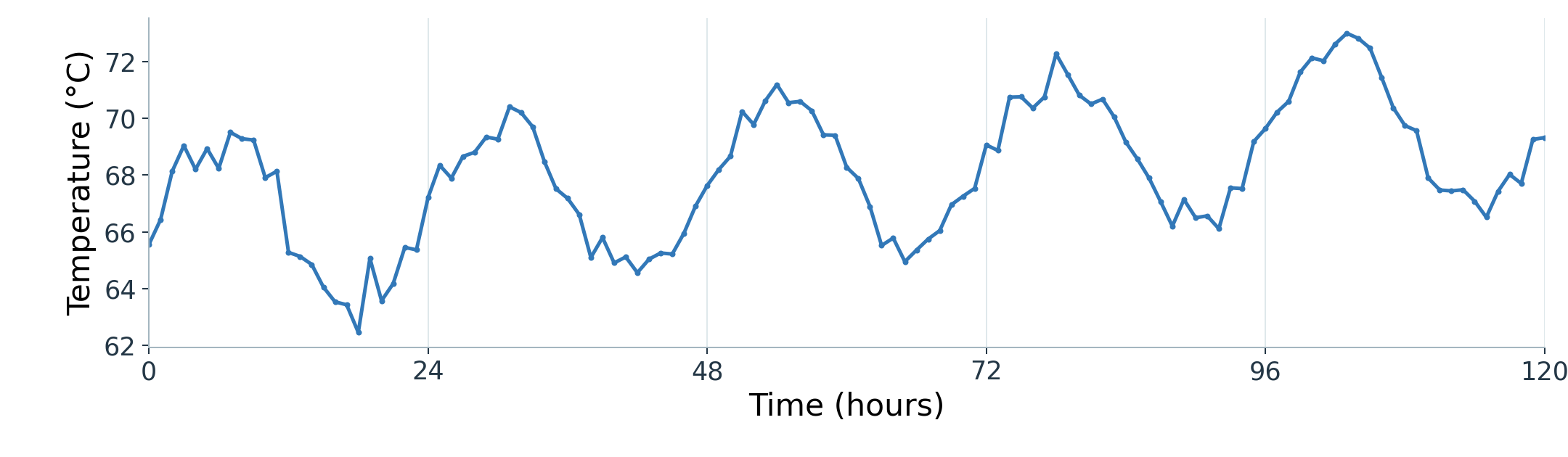
The line shows an overall rise, repeated peaks, and smaller irregular changes. Shuffling the readings would hide their order and change the apparent pattern. Before choosing a forecasting model, identify the sampling interval, units, and patterns in the observed history.
Decomposition: separating the patterns
Time-series decomposition estimates components that together describe an observed series. In an additive decomposition, the components add to the observation at each time:
y_t=T_t+S_t+R_t.
Here t identifies the time and y_t is the observed value.
- Trend, T_t: the underlying level and longer-term direction. This is shorthand for the trend-cycle component.
- Seasonality, S_t: variation that repeats at a regular interval, such as a daily operating cycle.
- Remainder, R_t: what remains after subtracting the estimated trend and seasonality.
The purpose is to separate long-term change from repeated variation, then examine what those components do not explain. Additive decomposition is suitable when seasonal fluctuations have roughly constant size. The components are estimates, so the result depends on the method used. Forecasting: Principles and Practice, time-series components.
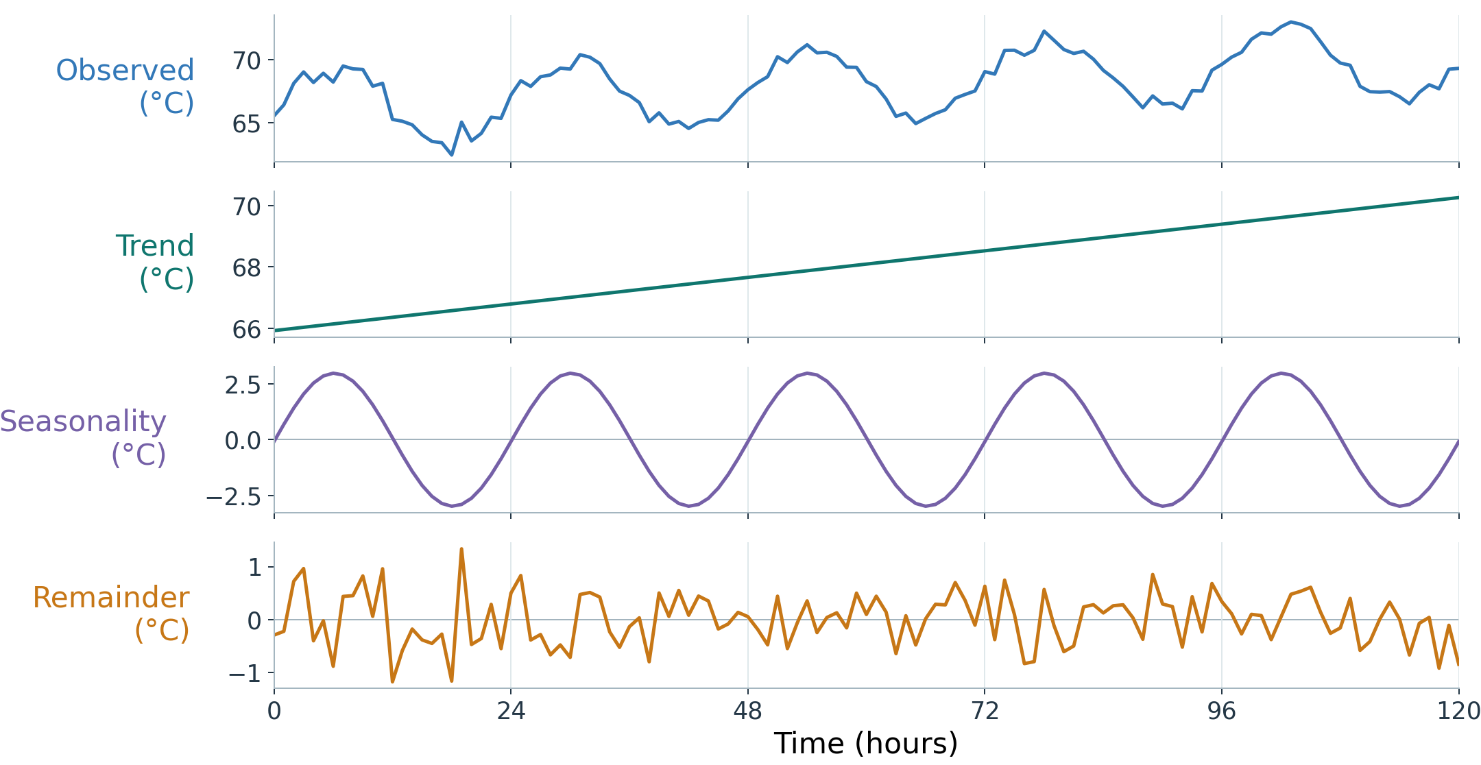
Read the panels at the same position along the time axis. The trend gives the underlying temperature level. The seasonal component adds or subtracts the contribution of the daily pattern. The remainder supplies the difference still needed to recover the observation. Negative seasonal or remainder values are adjustments to the level, not negative absolute temperatures. Check the axis values because the panels use different vertical scales.
For this illustration, a line and a 24-hour repeating pattern were fitted to the observed data, and the remainder was calculated by subtraction. The remainder is not necessarily random noise. It can contain unusual events or patterns the fitted components missed. Decomposition helps describe a series; it is not a required step for every forecasting model. When evaluating forecasts, estimate any decomposition used by the model from the history available at that forecast’s origin.
Lags: using earlier readings
Machine temperature often changes gradually, so recent readings may help predict the next one. Temporal dependence means observations at different times are statistically related. The relationship may also involve a daily pattern, and need not be causal.
A lag is a time offset from a stated reference time. In these slides, count back from the reading being predicted. To predict the next value after 10, 12, 14, lag 1 is 14, lag 2 is 12, and lag 3 is 10. For hourly data, lag 24 refers to 24 hours before the target.
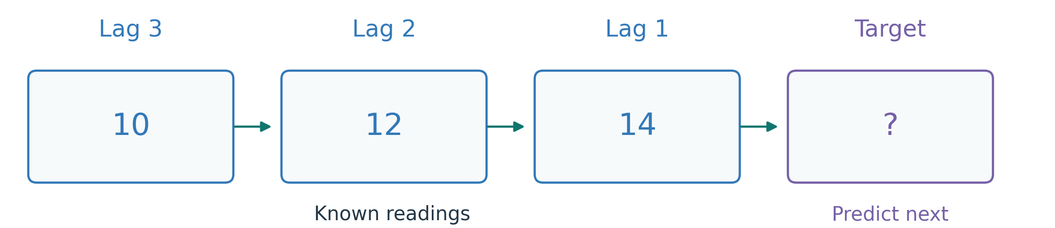
Practice: once 17 arrives, what are lag 1 and lag 2 when predicting the next reading?
Lag 1 is 17 and lag 2 is 14. The reference is the new, still-unknown target. This is the same convention used in the training table later.
Further detail: autocorrelation measures the linear relationship between a series and its own lagged values. A trend can also produce strong autocorrelation, and nonlinear dependence may not be captured. The short timeline explains positions; it does not establish a statistical relationship. Test whether lag inputs improve forecasts on later data.
I.B) Defining the Forecast
Lookback window, forecast origin, and horizon
Forecasting estimates future observations using information available when the prediction is made. Three terms specify the task:
- Forecast origin: the time at which the forecast is made.
- Lookback window: the history supplied as input.
- Forecast horizon: how far into the future the prediction extends.
For example, use the preceding 12 hours of temperature history to predict the next 6 hours. At hour 24, the lookback is the recent history ending at hour 24, while the six-hour forecast extends to hour 30. The actual readings after hour 24 are not yet available.
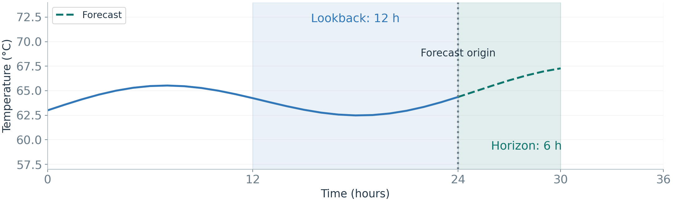
Choose the horizon from the decision. An operator responding in the next hour needs a different forecast from a planner preparing tomorrow’s schedule. A longer lookback is not automatically better: older data may add useful cycles or may describe conditions that no longer apply.
Variables and prediction steps
A univariate forecast uses a variable’s own history. A forecast with covariates adds related inputs, such as past RPM, load, or ambient temperature. Joint multivariate forecasting predicts several related variables together. These terms distinguish input choice from output choice; some sources use “multivariate” more broadly for models using several variables.
A one-step forecast predicts the next observation. A multi-step forecast predicts several future observations. A model can produce these together, or it can repeatedly use its own predictions as inputs. The repeated approach can accumulate errors because later predictions depend on earlier predicted values.
Every input must be available at the origin. A planned future load schedule may be available; the future load that eventually occurs may not be. State the target, sampling interval, horizon, and input availability before comparing models.
I.C) Forecasting Methods
The methods below differ in how they use history. They are alternatives to evaluate, not levels that must be completed in order. A baseline is a simple comparison method that helps establish whether a more complex model adds value.
How a model learns to forecast
A model is a rule or learned relationship that turns inputs into a prediction. Inputs, also called features, are the information supplied to it. The target is what it tries to predict.
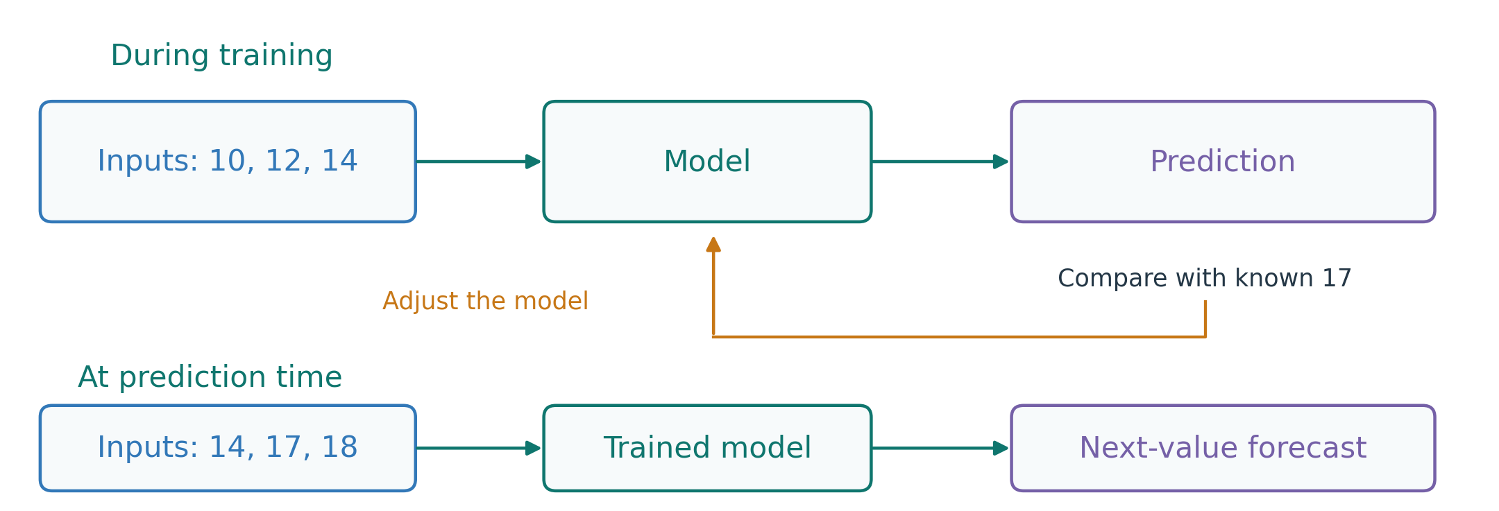
Training uses historical examples with known targets to adjust the model’s settings. For example, readings 10, 12, 14 can be paired with the next recorded reading, 17. Comparing a model’s prediction with that known target helps guide learning. Many examples are needed; the small table is only an illustration.
At prediction time, the model receives the latest history, such as 14, 17, 18, while the next reading remains unknown. It applies what it learned to estimate that value. Learned settings are often called parameters or weights. A fixed rule, such as the naive forecast below, does not need learned parameters.
Comparing forecasting approaches
The task stays the same across these approaches: use available history to predict a future reading. What changes is how the method uses that history.
- Simple rules repeat a recent value or a value from the previous cycle.
- Statistical models describe patterns such as the recent level and relationships with earlier values or errors.
- Lag-feature models use a table of past readings and other available inputs.
- Sequence models learn patterns from readings in time order.
- Pretrained models reuse patterns learned from many other series.
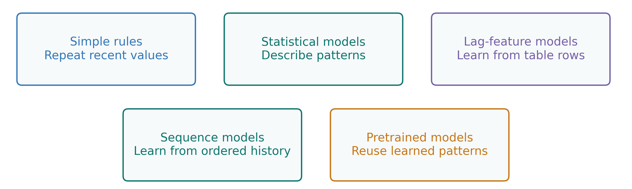
These are alternatives to compare, not steps in a required pipeline. Start with a simple baseline, then check whether a more complex method improves forecasts on later data for the same target and horizon. The next sections explain each approach.
Naive and seasonal-naive baselines
A naive forecast repeats the latest observed value. If the current reading is 15, its next forecast is 15. A seasonal-naive forecast repeats the value from the corresponding position in the last known cycle. With hourly data and a daily cycle, tomorrow’s forecast for a particular hour uses that hour’s value from the previous day. In decomposition terms, this baseline reuses the seasonal pattern.
Both are transparent and inexpensive. They cannot anticipate a new operating regime, and neither explicitly models a new trend. Compare other models with these baselines using the same target, horizon, and evaluation periods.
Smoothing: estimating the recent level
A trailing moving average averages a recent window of observations. Simple exponential smoothing combines the previous level and the latest observation using weighted averaging. For a previous level of 70°C, a new reading of 80°C, and a weight of 0.2 on the new reading, the updated level is 0.8(70)+0.2(80)=72°C. This becomes the next forecast. In general:
\ell_t=\alpha y_t+(1-\alpha)\ell_{t-1}, \qquad \hat y_{t+1}=\ell_t.
Here y_t is the latest reading, \ell_{t-1} is the previous estimated level, \ell_t is the updated level, and 0<\alpha<1 controls the update weight. A larger \alpha responds more strongly to the latest reading. Older observations receive geometrically decreasing weights. Simple exponential smoothing is a level-only method; extensions can include trend and seasonality. Forecasting: Principles and Practice, simple exponential smoothing.
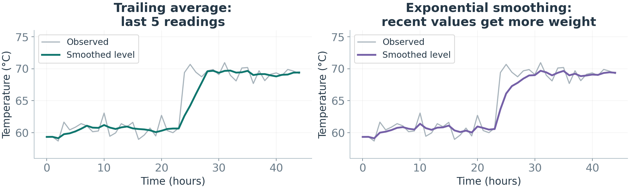
The plotted estimates already include the reading at their time. They are therefore smoothed levels, not forecasts made before that same reading arrived. To predict y_t, use the earlier level \ell_{t-1}. After observing y_t, update the level and use it to predict y_{t+1}. This timing distinction prevents an apparently accurate smoothing curve from being mistaken for forecasting performance.
Stationarity: whether the pattern stays stable
Before introducing ARIMA, consider whether the pattern being modeled stays reasonably stable. Informally, stationarity means that the average, spread, and relationships between readings at a fixed time gap remain stable over time.
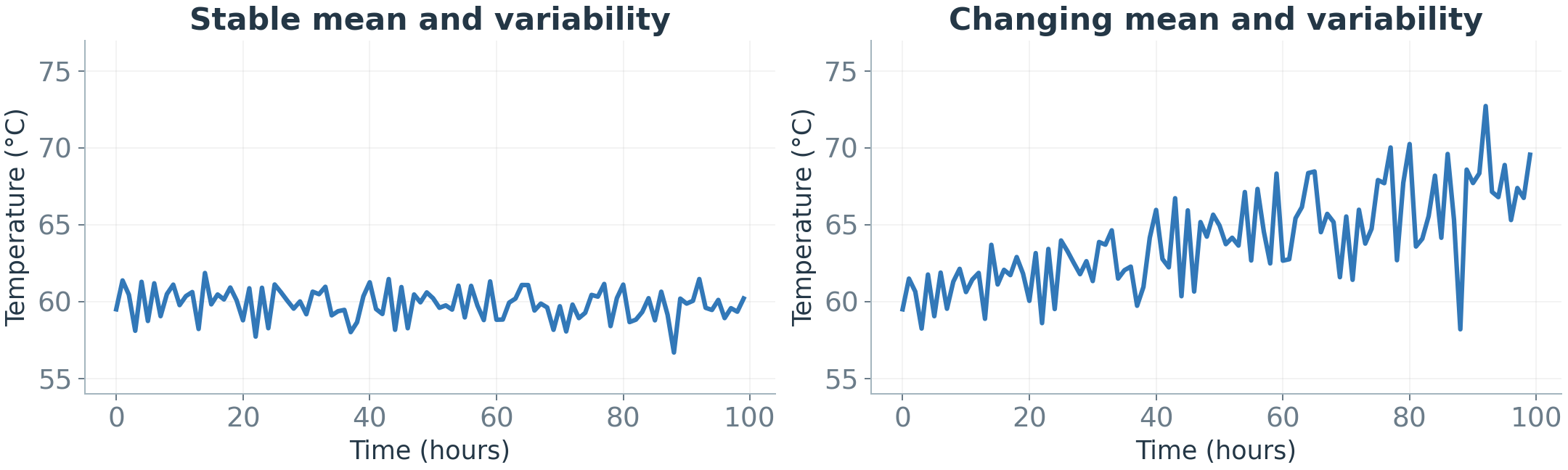
The left panel illustrates a stable level and spread; the right panel shows both changing. A short graph can suggest instability, but it cannot prove stationarity.
Further detail: a weakly stationary series has a constant mean and variance, and its covariance between observations depends on their time gap rather than their calendar date. Covariance describes how observations vary together.
Differencing stops looking at the value itself and looks at how much it changed. Instead of asking what the temperature is, it asks how much the temperature changed from the previous time. A first difference records the change between consecutive readings:
\Delta y_t=y_t-y_{t-1}.
For readings 10, 12, and 15, the differences are 2 and 3. Why does this help before ARIMA? Consider 10, 12, 14, 16, 18: the original series clearly keeps increasing, but its differences are 2, 2, 2, 2, a stable pattern. When a series keeps rising because of a trend, differencing can remove that changing level and reveal a more stable pattern underneath, which is what ARIMA needs. Differencing can reduce some trends, but it does not automatically correct changing variance, sensor problems, or every change in behavior. Inspect the transformed series and choose transformations for the model being used. The ARIMA model below assumes the differenced series behaves stably. Forecasting: Principles and Practice, stationarity and differencing.
ARIMA: past values, differencing, and past errors
A forecast error is actual minus forecast. The errors ARIMA uses are past ones: an earlier forecast said 70, the actual reading was 72, so that forecast missed by +2. A past prediction mistake like this is also called a residual. ARIMA can learn how such earlier misses relate to later values; a positive error does not always imply an upward correction.
ARIMA combines three components:
- AR, autoregression: uses previous values of the modeled series.
- I, integration: indicates differencing of the original series before modeling.
- MA, moving average: uses past model errors, also called innovations.
The simplest useful version, ARIMA(1,1,1), can be written for the differenced series y'_t, meaning the changes between consecutive readings:
y'_t=c+\phi_1\,y'_{t-1}+\theta_1\,e_{t-1}+e_t
Read it term by term. c is a constant level for the changes. \phi_1\,y'_{t-1} says: use the previous change; this is the autoregressive, AR, part, and \phi_1 is a learned coefficient that scales it. \theta_1\,e_{t-1} says: use the previous forecast error; this is the MA part, with its own learned coefficient \theta_1. Finally e_t is the new error at time t, the part the model cannot predict. Training estimates c, \phi_1, and \theta_1 from historical data.
In ARIMA(p,d,q), p specifies the number of past-value terms, d the order of differencing, and q the number of past-error terms. For example, ARIMA(2,1,1) models the once-differenced series using two of its previous values and one previous error term. The formula above is the p=1, d=1, q=1 case. Predictions of changes are converted back to the original measurement scale.
The MA component is not a rolling average of sensor readings. ARIMA describes linear temporal relationships, and the differenced process should have reasonably stable behavior. Its settings still require evaluation; differencing is not a general remedy for every type of change. Forecasting: Principles and Practice, ARIMA models.
Lag features: turning a sequence into training rows
A lag-feature table pairs known history with a later target. This allows ordinary supervised models, such as linear regression, random forests, or gradient boosting, to make forecasts.
Practice: from 10, 12, 14, 17, 18, form two training rows, each using three earlier readings to predict the next reading.
| Lag 3 | Lag 2 | Lag 1 | Target |
|---|---|---|---|
| 10 | 12 | 14 | 17 |
| 12 | 14 | 17 | 18 |
Here the lag columns are named relative to the target time. For target 17, lag 1 is 14. Once 18 is observed, the next input window is 14, 17, 18, while its future target remains unknown. This is the same idea as the earlier lag timeline, with the reference time stated explicitly.
Rolling features summarize a past window, for example its mean. Calendar features describe known timing, such as hour or weekday. Construct each feature using only information available at that row’s forecast origin.
Random forests combine the predictions of multiple trees. Gradient boosting adds trees that improve the current fit. These methods can capture nonlinear feature relationships, but the table must provide the relevant temporal information. Trees do not automatically understand time order and usually extrapolate trends poorly beyond the training range.
Sequence models: learning from ordered history
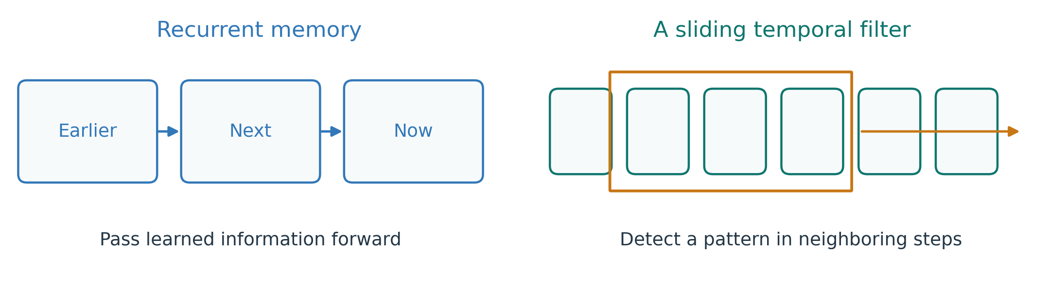
Keep the earlier task in mind: use 10, 12, 14 to predict the next reading. A lag table supplies selected past values and summaries. A sequence model processes readings in time order and learns patterns across that history. A recurrent neural network (RNN) passes a learned state from one step to the next. An LSTM, or long short-term memory network, uses gates to control what information is retained or changed. These gates can help with longer relationships but do not guarantee perfect memory.
A temporal convolution applies learned filters to neighboring time steps. A filter might respond to a short vibration burst. Stacking filters can cover longer histories; a causal design avoids using future readings when producing a prediction.
Attention: connecting distant times
A useful pattern may come from yesterday’s operating cycle as well as the latest few readings. For the same next-reading task, a model may need information from both parts of the history.
Attention learns how much information to combine from different observed positions when forming a representation. A Transformer uses attention to connect relevant parts of a sequence, including positions far apart. This can help compare similar operating cycles without passing all information through each intervening recurrent step. Long histories can still require substantial memory.
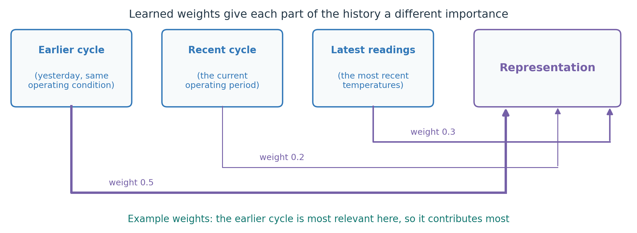
In the figure, the three parts of the history have concrete meanings: the earlier cycle is yesterday at the same operating condition, the recent cycle is the current operating period, and the latest readings are the most recent temperatures. Attention gives different importance, called weights, to these parts. In the example the weights are 0.5 for the earlier cycle, 0.2 for the recent cycle, and 0.3 for the latest readings, so the earlier cycle contributes most because it is most relevant to the current situation. These example weights are illustrative; a real model computes its own.
Attention weights are not proof of a causal explanation. All these models must obey the same information boundary: actual future readings cannot enter a forecast. Their value should be established against simpler methods on later data.
Pretrained forecasting models
A pretrained model has already learned settings, called weights, from earlier training. We can reuse those settings for a new task. A time-series foundation model is pretrained on many series for broad reuse, including application or adaptation to new forecasting tasks. Zero-shot forecasting uses a new series as input context without updating the pretrained weights on that target series. Zero-shot does not mean forecasting without any history.
TimesFM and Chronos are examples of this approach. Model versions differ in supported inputs and outputs. Check whether the selected version accepts the variables and horizon required by the task. Reusing a pretrained model may reduce task-specific training, but it does not remove the need for local evaluation or comparison with a baseline.
I.D) Evaluating Forecasts
Temporal splits: learn, choose, and assess
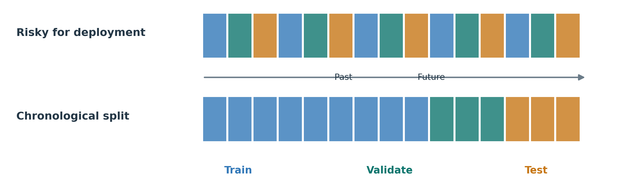
For a model intended to forecast future operation, evaluation should follow time: train on earlier data, choose settings using later validation data, and assess the selected model on a separate final test period. Randomly mixing nearby observations can expose the model to future conditions or closely related examples.
Leakage: information used before it is available
In this forecasting setting, data leakage occurs when a prediction uses information unavailable at its forecast origin. A centered rolling mean includes observations on both sides of a time, so it can include future readings. A scaler fitted to the entire dataset uses statistics from future validation or test periods.
Past observations can legitimately provide context for later predictions. The restriction concerns availability, not whether a value mentions a future date. For example, a forecast of tomorrow’s weather issued today can be used today; tomorrow’s actual observed weather cannot.
What to check: reconstruct what the system knew at each origin, including when sensor readings, labels, forecasts, and schedules became available. Apply that check to features and preprocessing as well as model fitting.
Forecast errors and their units
Let y_t be the actual value and \hat y_t the forecast made before it was observed. The forecast error is actual minus forecast:
e_t=y_t-\hat y_t.
For the slide’s energy example, actual values are 10, 20, 30 kWh, while forecasts are 12, 18, 36 kWh. The signed errors are −2, 2, −6 kWh, and the absolute errors are 2, 2, 6 kWh.
| Metric | Definition | Worked result |
|---|---|---|
| Mean absolute error, MAE | \frac{1}{n}\sum_{t=1}^{n}\lvert y_t-\hat{y}_t\rvert | (2+2+6)/3=3.33 kWh |
| Root mean squared error, RMSE | \sqrt{\frac{1}{n}\sum_{t=1}^{n}(y_t-\hat{y}_t)^2} | \sqrt{(4+4+36)/3}=3.83 kWh |
| Mean absolute percentage error, MAPE | \frac{100}{n}\sum_{t=1}^{n}\left\lvert\frac{y_t-\hat{y}_t}{y_t}\right\rvert | (20+10+20)/3=16.7\% |
RMSE gives larger errors more influence because it squares them before averaging. MAE and RMSE retain the target’s units. MAPE is undefined when an actual value is zero and unstable near zero. It also requires a meaningful measurement zero, which energy has but Celsius temperature does not. Compare metrics for the same target, horizon, and periods. Forecasting: Principles and Practice, forecast accuracy.
Walk-forward validation
Walk-forward validation repeats this process at several forecast origins. At each origin, use the available history, generate the required forecasts, and record the later errors. The training history may expand or use a rolling window. Refit the model according to the intended update policy; a fixed forecasting rule may only need its input history refreshed. Forecasting: Principles and Practice, time-series cross-validation.
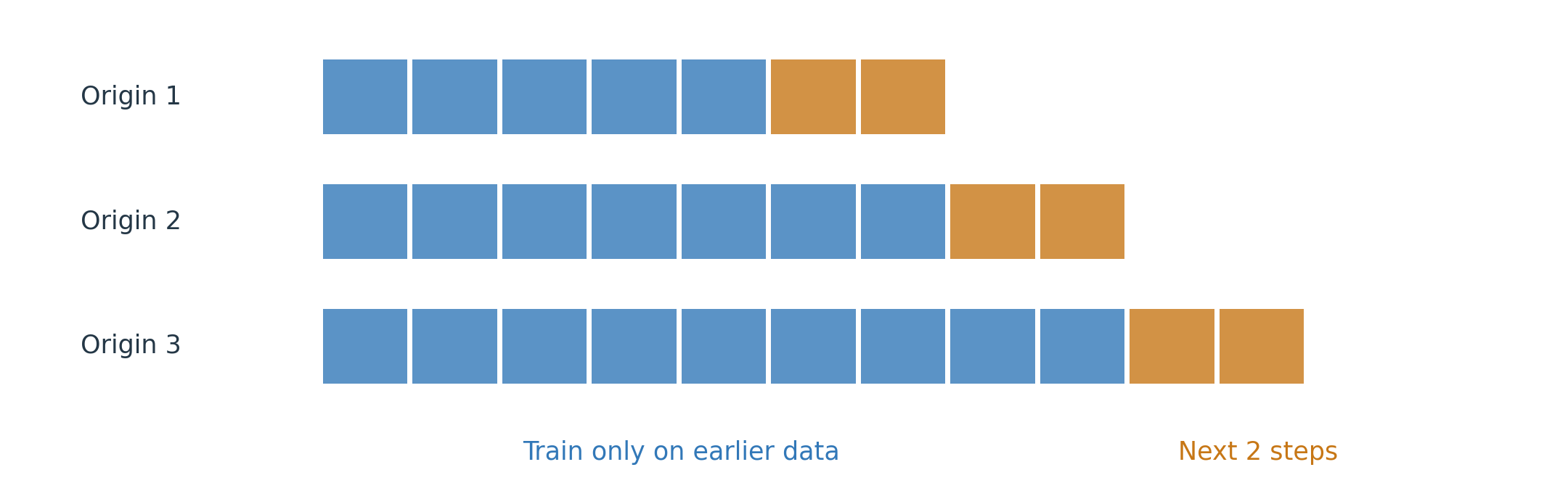
Keep the final test period separate from the origins used to select the model. Fit learned preprocessing, such as scaling, using each origin’s permitted training data. With multi-step targets, make sure training labels do not cross into the validation or test period. Add a gap where overlapping targets would otherwise leak information. If the intended use is a new machine, a machine-level split may also be needed.
Practice: use a naive one-step forecast for the sequence 10, 12, 14, 17, 18. Evaluate the forecasts made immediately after observing 12, after 14, and after 17.
| Origin | Forecast | Next actual value | Absolute error |
|---|---|---|---|
| After 12 | 12 | 14 | 2 |
| After 14 | 14 | 17 | 3 |
| After 17 | 17 | 18 | 1 |
The MAE is (2+3+1)/3=\mathbf{2} units. The last forecast can use 17 because it has become available by that origin. It could not be used for the earlier forecasts.
Prediction intervals: a range for a future observation
A prediction interval expresses uncertainty about a future observation. The slide gives a forecast of 75°C, with an illustrative 90% prediction interval of 68 to 82°C. Over repeated comparable forecasts, a well-calibrated 90% interval should contain about 90% of the actual future observations.
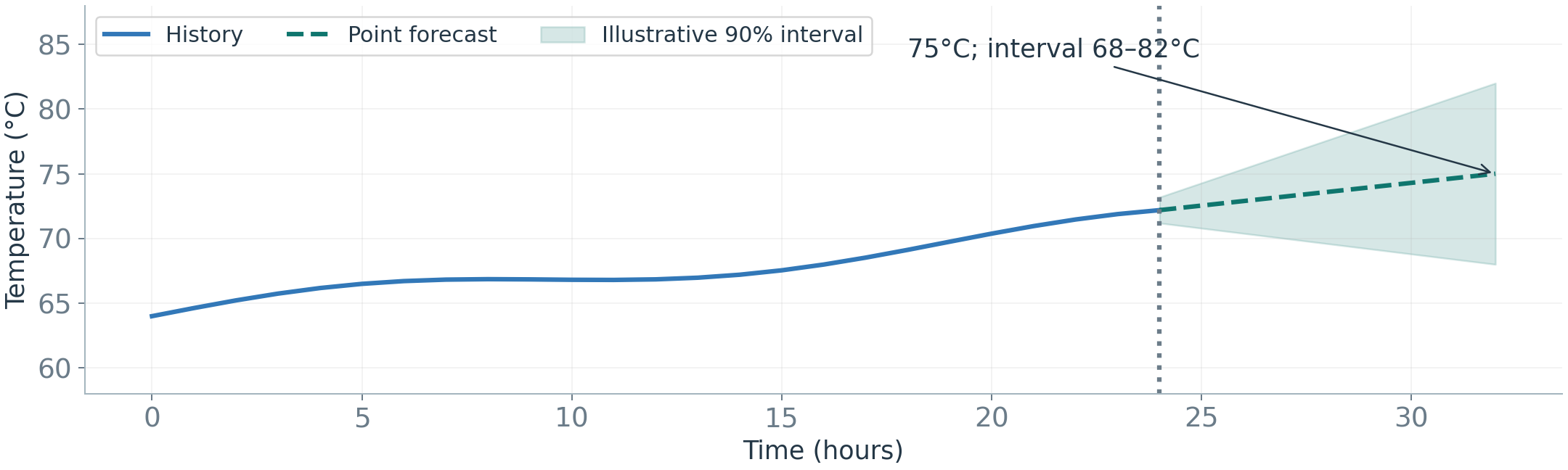
Observed coverage is the proportion of evaluated observations inside their intervals. If 90 of 100 observations are inside, coverage is 90%. Check coverage together with interval width: an extremely wide interval may cover almost everything while providing little useful guidance. Also check relevant operating conditions and horizons separately.
A prediction interval is not a guaranteed safe operating range, nor is it a confidence interval for an estimated model parameter. A forecast can be statistically plausible and still describe an undesirable machine condition.
I.E) Distribution Shift and Adaptation
Monitoring forecast accuracy
A model that performed well during testing may become less accurate in daily use. Model degradation means predictive performance worsens over time. Compare forecasts with measurements when those measurements arrive. Monitor error by horizon and operating condition, because a single overall average can hide a problem affecting only part of the operation.
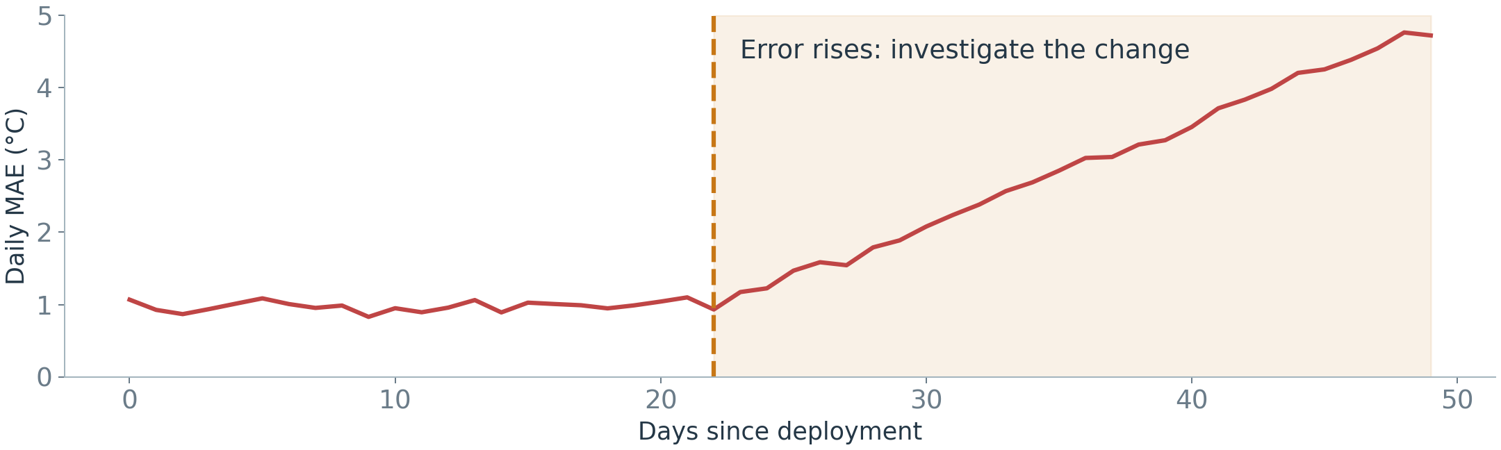
Rising error is a reason to investigate. It may reflect new conditions, a changed relationship, missing information, or a sensor issue. Input shift can be detected before target labels arrive, but input shift alone does not prove that prediction accuracy has fallen.
Covariate shift and concept drift
To investigate rising forecast errors, ask two questions: are the operating conditions different, or does the machine behave differently under the same conditions? A deployed model may encounter either change, or both.
- Covariate shift: the input distribution changes while the conditional target relationship stays the same. For example, high RPM becomes more common, but fuel use at a given RPM and load follows the previous relationship.
- Concept drift, as used here: the conditional relationship changes. The same RPM and load now correspond to higher fuel use.
Optional aside, for readers familiar with probability notation: writing inputs as X and the target as Y, P(X) describes the input distribution, and P(Y\mid X) describes the target distribution for given inputs. Covariate shift changes P(X) while preserving P(Y\mid X); concept drift here changes P(Y\mid X). Both can occur together. Terminology varies: drift literature also uses virtual drift and real drift for these distinctions, and sometimes uses “concept drift” more broadly. See Gama et al., reference 2.
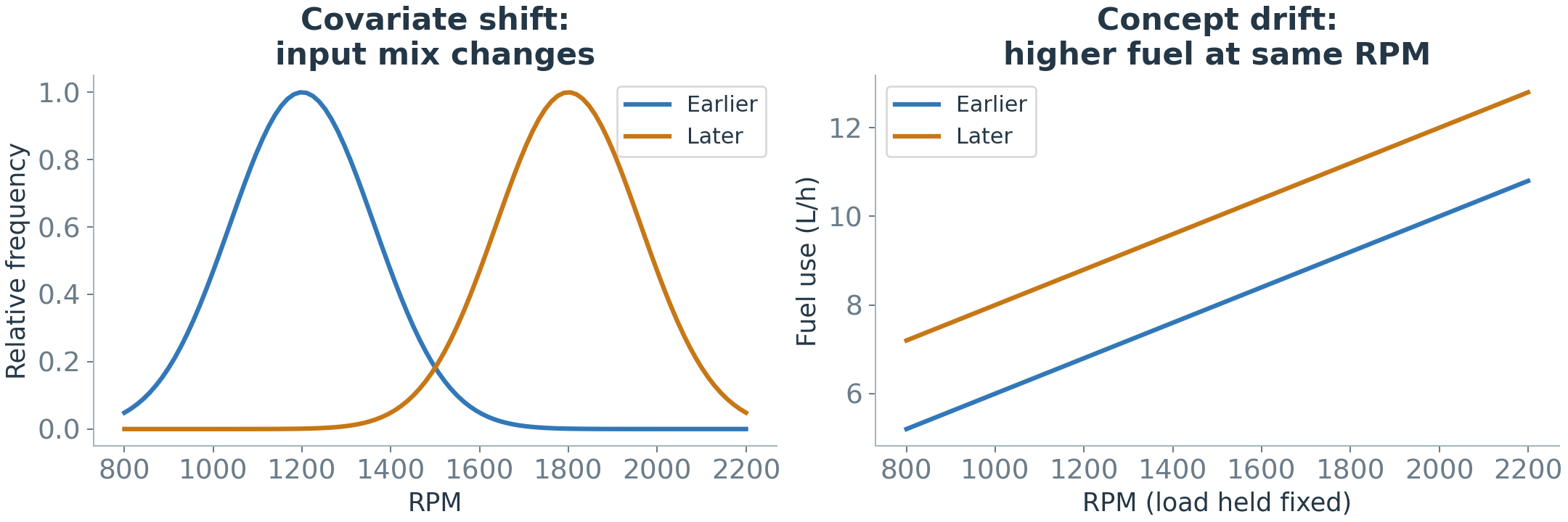
A changing output average alone does not identify the cause. Monitor inputs and prediction errors, and compare comparable operating conditions. A predictable seasonal pattern can make a series non-stationary without showing that a learned relationship has failed.
How changes appear
The slides distinguish four schematic patterns:
- Sudden: one regime abruptly replaces another, as might happen after a sensor replacement.
- Gradual: old and new regimes coexist during a transition.
- Incremental: the relationship moves continuously, as gradual wear might produce.
- Recurring: a previous regime returns.
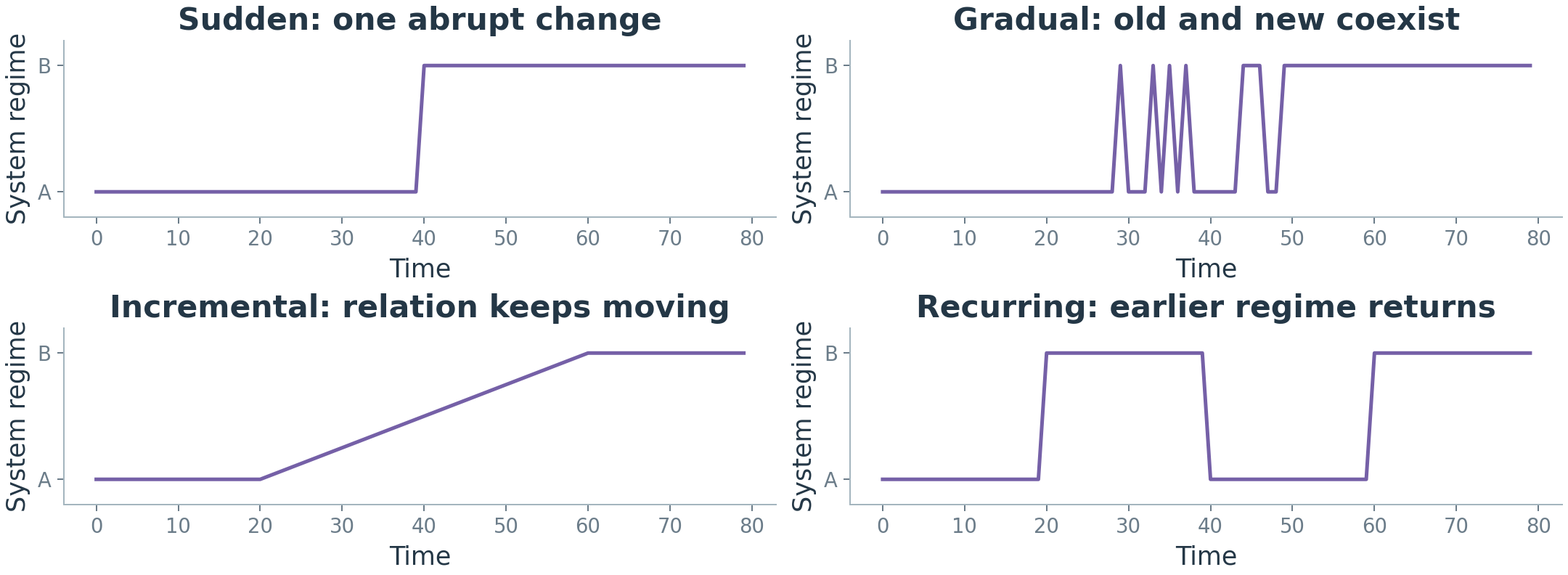
“Gradual” in everyday speech can mean any slow change. In this classification, it specifically describes coexistence during a transition, whereas continuous movement is called incremental. The diagrams describe change patterns, not their physical causes.
Practice: which pattern fits a sensor replaced in one step? Which fits a machine that wears a little more each month?
A one-step replacement could produce a sudden change. Steady movement associated with wear could produce an incremental change. These examples illustrate the timing of a change; the trace alone does not establish its cause.
Deciding how to adapt
Four update strategies appear in the slides:
- Periodic retraining: refit on a schedule.
- Sliding window: fit using only recent history.
- Drift-triggered retraining: investigate a detected change, then refit when appropriate.
- Online learning: update incrementally as suitable training examples arrive.
These choices can be combined. A sliding window specifies which data to use, while periodic or triggered retraining specifies when to update. Recent windows can adapt to new behavior but lose older examples of rare valid regimes. Validate updates on later data after investigating why the system changed.
Practice: forecast error increases after a sensor replacement. What should be checked before retraining?
Check units, calibration, timestamps, missing readings, and whether the physical process or operating policy also changed. Compare other sensors and maintenance records. Retraining on a unit or calibration error could make the model reproduce the error instead of correcting the data problem.
Forecasting now provides an expectation that can support the next part of the lecture: comparing what happened with what was expected.
II.A) Understanding Anomalies
An anomaly is a reason to investigate
An anomaly is an observation or pattern that differs meaningfully from expected behavior for a task and context. A temperature spike could reflect a fault, a sensor error, or a valid operating event. Detection identifies something to examine; it does not establish why it happened.
A normal reference is the evidence used to describe expected behavior. It might be a confirmed healthy operating period, typical values and spread, similar trusted examples, or a forecast. A useful reference covers relevant loads and environments. A reference containing hidden faults or only low-load operation can be misleading.
Anomaly detection is difficult because faults may be rare, labels may be scarce or delayed, future faults may differ from known ones, and valid operating conditions may change. An unlabeled dataset does not remove the need for assumptions: a detector may assume, for example, that anomalies are rare or structurally different from most observations.
Point, contextual, and collective anomalies
A point anomaly is an individual observation that is unusual relative to its reference. A contextual anomaly is unusual under particular conditions, such as a temperature that is ordinary at midday but unexpected at night. A collective anomaly is an unusual group or sequence, even when its individual values appear plausible. These distinctions follow the framework in Chandola et al.’s survey.
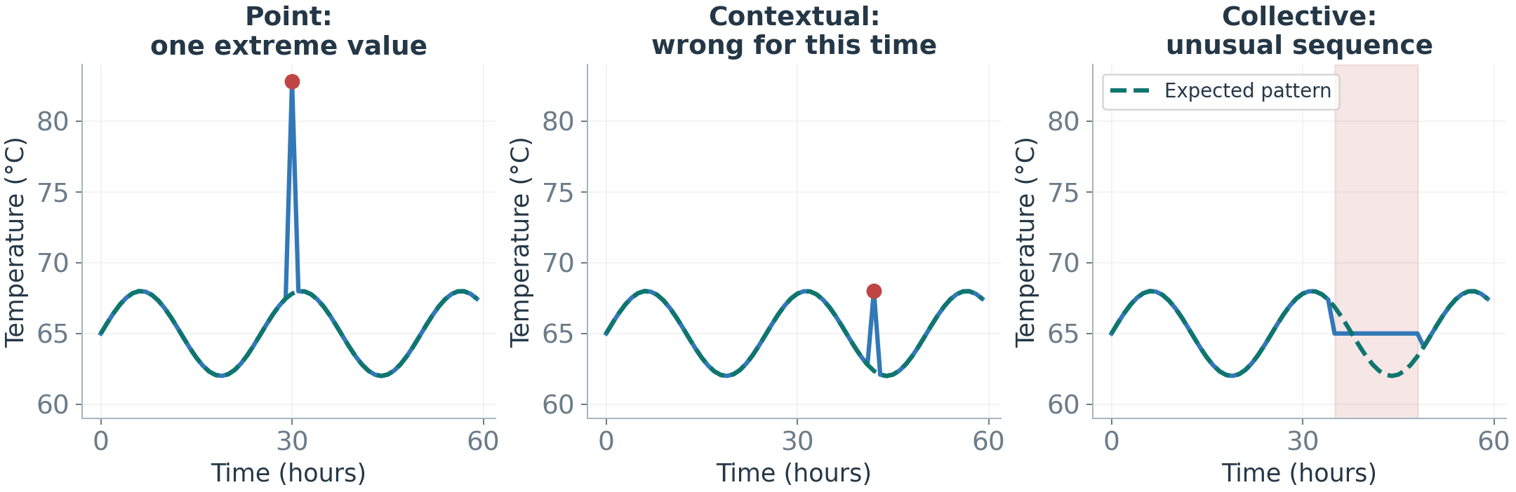
In the collective example, a flat trace may be suspicious because a healthy sensor normally oscillates. A threshold applied independently to each value could miss the problem. Choose inputs that preserve the evidence the detector needs, such as recent history or operating context.
Multivariate anomalies: unusual combinations
A temperature of 72°C may be normal at high RPM but unusual at 1,000 RPM. In the illustrative relationship from the slides, expected temperature is approximately 35+0.02\times\mathrm{RPM}, so 1,000 RPM corresponds to about 55°C. The 72°C observation is therefore unexpected for that condition, even if it is inside the overall temperature range.
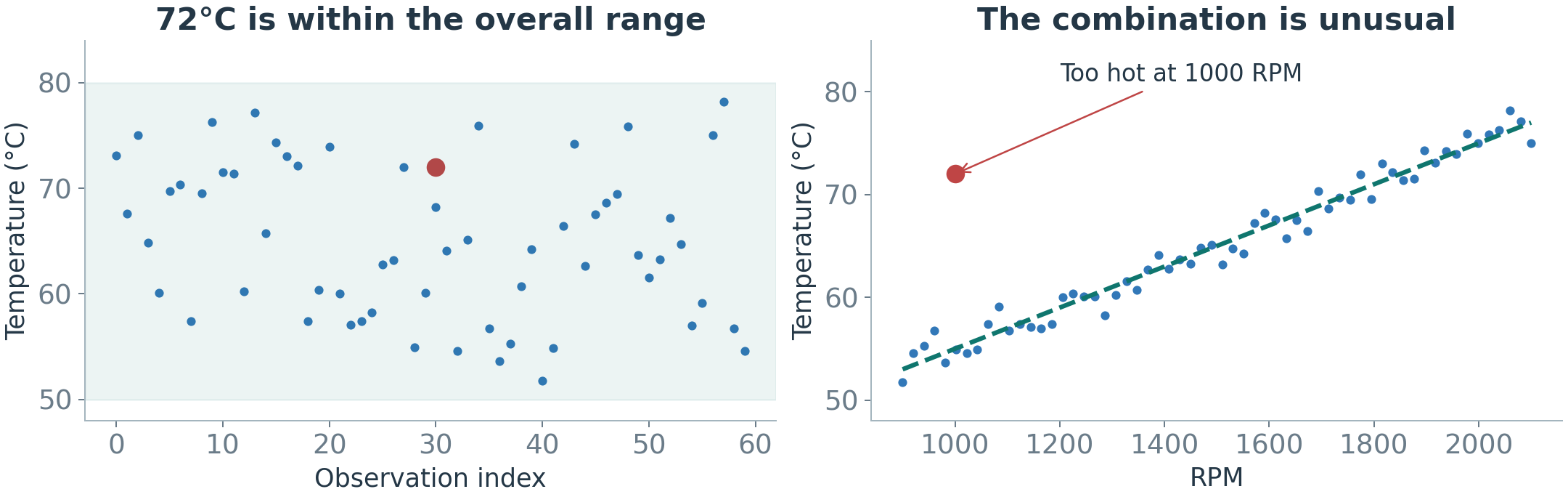
Univariate detection examines one variable. Multivariate detection can examine several variables and their relationships. Separate sensor limits may miss an inconsistent combination. Load and ambient temperature may also matter, so the RPM-temperature example illustrates the principle rather than a complete machine model.
II.B) Defining Normal Behavior
What training labels are available?
A label records what an example represents, such as normal operation or a confirmed failure. The available training evidence determines the learning setting.
| Setting | Normal labels | Anomaly labels | What the model learns |
|---|---|---|---|
| Supervised | Yes | Yes | Differences between known classes |
| Normal-only / one-class | Yes, or trusted normal data | Usually no | The region or patterns associated with normal behavior |
| Unsupervised | No | No | Unusual structure relative to assumptions about the data |
Terminology varies. Here, one-class training describes learning from trusted normal examples. In other parts of machine learning, “semi-supervised” usually means combining labeled and unlabeled examples. A supervised detector may miss a new fault unlike its labeled examples; an unsupervised detector may flag a rare but valid regime. Reliable event labels remain valuable for evaluation even when they are not used for training.
For example, supervised training might use 900 normal examples and 100 failure examples. Normal-only training could use 900 confirmed healthy examples. Unsupervised training might use 1,000 readings with no labels. The same algorithm family can be used in different settings, depending on the data supplied.
From an unusualness score to an alert
An anomaly score describes how unusual an observation appears under the detector. A threshold turns that score into an alert decision. In the slide example, higher scores mean more unusual behavior, and score > 0.70 triggers an alert.
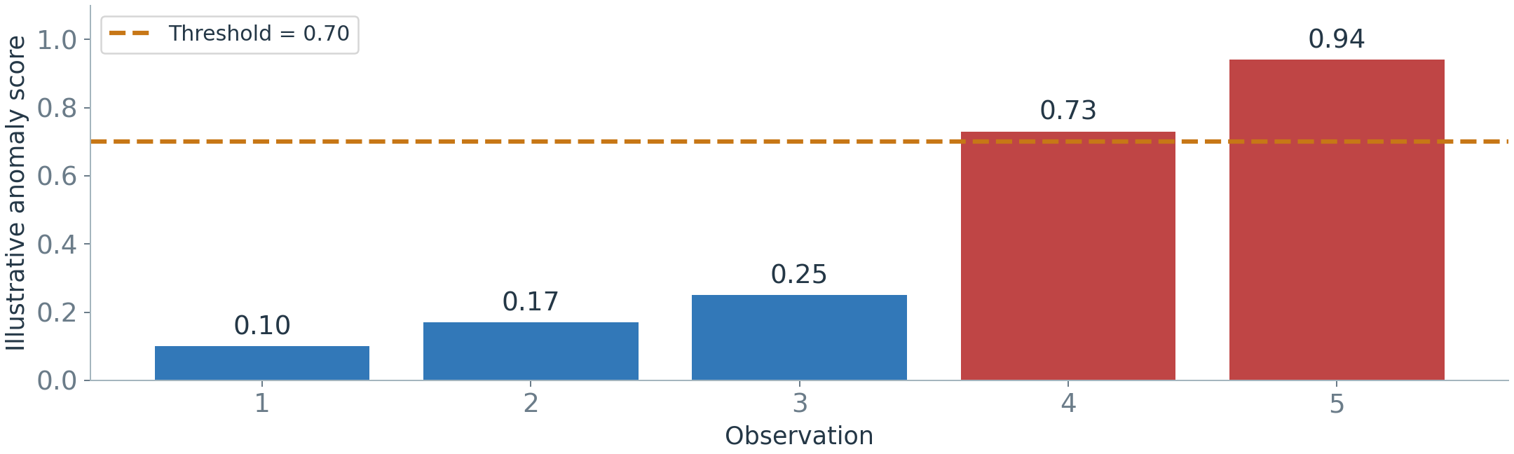
A score of 0.94 does not automatically mean a 94% probability of failure. Some algorithms use scores outside zero to one, and some implementations assign lower scores to more unusual examples. Check the convention before choosing a threshold.
A fixed engineering rule may return an alert directly, without a separate continuous score.
What does each detection method check?
Each method compares observations with a reference. The following questions match the order of the method explanations:
- Known limits: does a reading cross a known engineering limit?
- Statistical reference: is a reading far outside the usual range for these operating conditions?
- Forecast error: is the observed value far from a forecast made earlier?
- Neighbor distance: are even its nearest reference points far away?
- Local density: is the area around this point less crowded than the areas around its neighbors?
- Isolation: can a few random splits separate this point from the others?
- Reconstruction error: does the rebuilt input differ greatly from the original input?
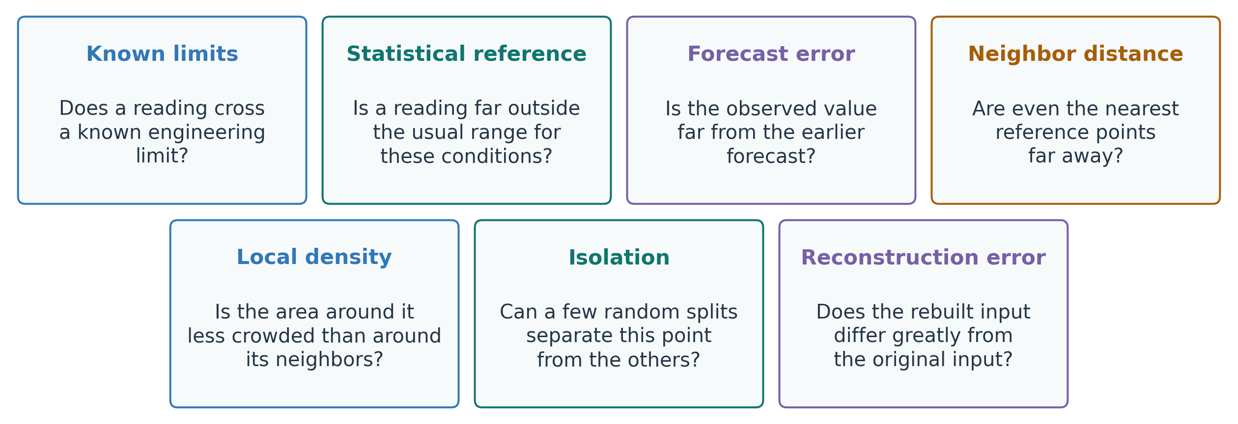
These are different checks, not mutually exclusive categories. A forecast can use several sensors, and an autoencoder can reconstruct an entire time window. Choose a comparison that retains the evidence needed to detect the problem.
II.C) Anomaly Detection Methods
Rules: checking a known limit
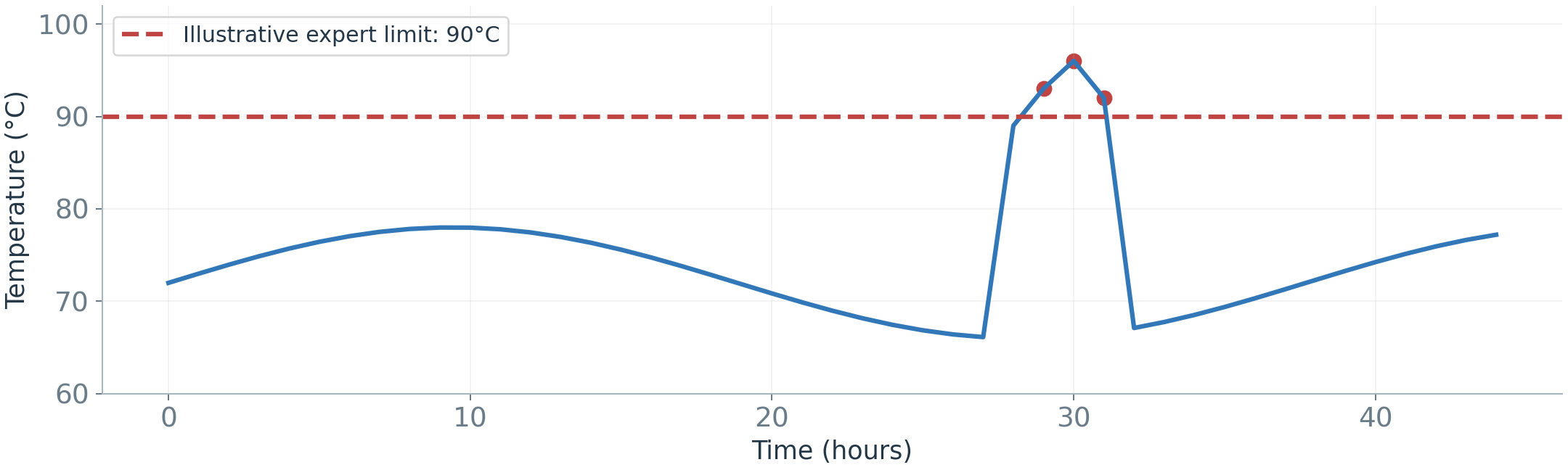
The first question in the overview is whether a reading crosses a known engineering limit.
A rule such as temperature > 90°C → alert is clear and inexpensive. Its threshold must come from the actual equipment and purpose; 90°C is only the slide’s illustrative value. A fixed limit may miss contextual problems or produce unnecessary alerts in valid operating regimes.
Statistical references: checking the expected range
The next question is whether a reading is far outside the usual range for comparable conditions. Unlike an engineering limit, this reference is estimated from data describing expected operation. A statistical method compares a reading with a reference distribution. Standard deviation measures spread around the mean. A z-score expresses how far a value is from that mean in standard-deviation units:
z=\frac{x-\mu}{\sigma}.
For reading x=86°C, reference mean \mu=70°C, and reference standard deviation \sigma=4°C:
z=\frac{86-70}{4}=4.
The reading is 16°C above the mean, or four standard deviations. The illustrative three-standard-deviation limits are 70-3(4)=58°C and 70+3(4)=82°C.
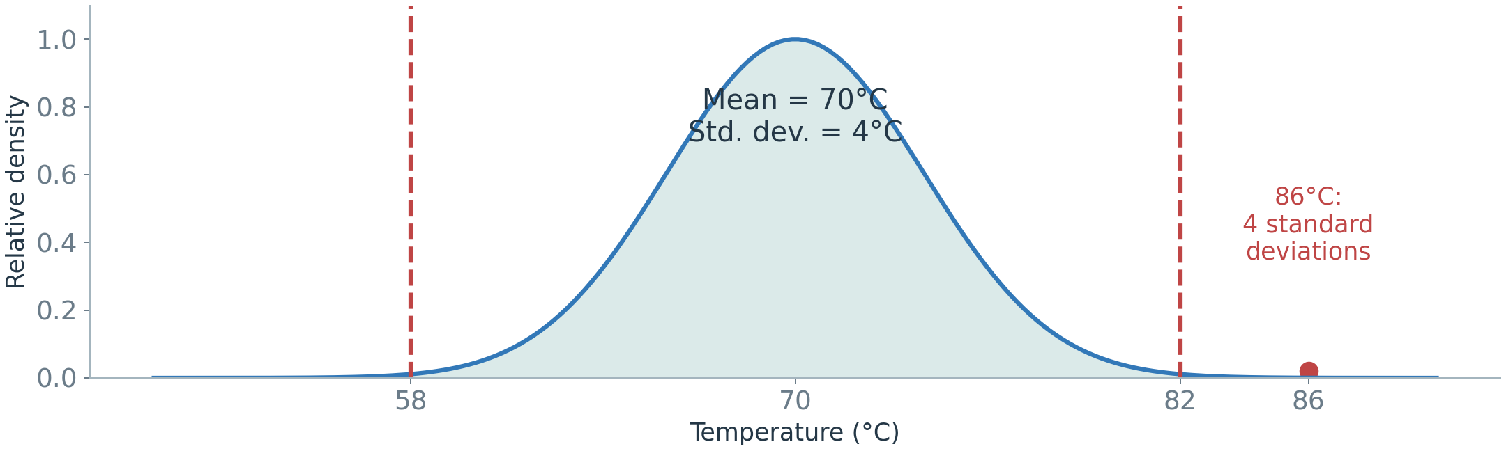
A three-standard-deviation rule is not universal. Its probability interpretation needs distributional assumptions. Skewed data, contaminated history, and mixed operating regimes can make one mean and spread misleading. Quantiles or robust summaries may be more appropriate. Estimate the reference using permitted training or calibration data, not the final test period.
Forecast error: comparing expected and actual
This method connects anomaly detection to Part I. A forecasting detector predicts a reading before it arrives, then compares the observation with the forecast. For a forecast of 70°C and an actual value of 75°C, the absolute error is 5°C. This is a simple anomaly score. Judge it against usual forecast errors: 5°C is more unusual when errors are typically around 1°C than when they are typically around 5°C.
Further detail: a scale-aware alternative is
s_t=\frac{|y_t-\hat y_t|}{\hat\sigma_t},
where \hat\sigma_t>0 estimates the expected error spread for the operating context. A 5°C error is more unusual when normal forecast errors are small than when they are routinely large. Estimate that spread without using the future observations being assessed.
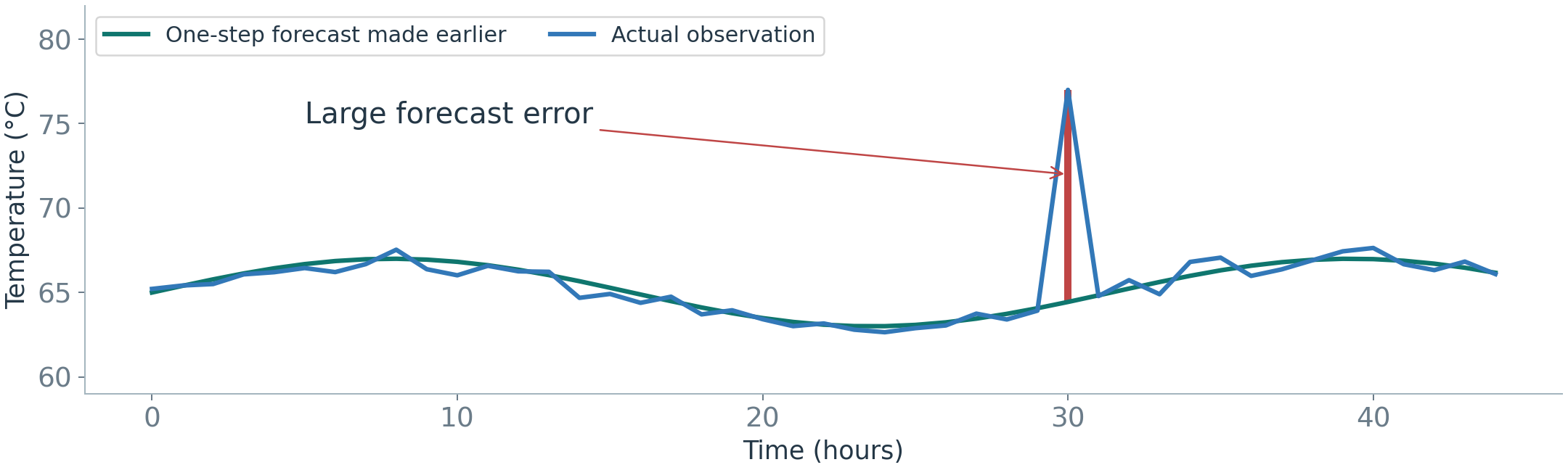
Poor forecasting, missing inputs, or drift can raise the score without a physical fault. A model that adapts too quickly can instead follow a developing fault and reduce the discrepancy. Evaluate both the forecasting reference and the resulting detector. The monitored quantity here is an out-of-sample forecast error; it is not a training residual used as if it were an unseen prediction. Like decomposition, this compares observations with an expected pattern. However, a forecast error is computed from a prediction made before the observation arrives; it is not the same quantity as a retrospective decomposition remainder.
Nearest neighbors: looking for similar examples
A k-nearest-neighbor (kNN) detector can score a reading by its distance to the kth nearest reference point. Here k is the chosen number of neighbors. A large distance means the model must look farther to find similar examples.
In the slide illustration, k=3. Blue points are reference observations; the red point is a new observation. The circle reaches the third-nearest reference point. A larger circle gives a larger distance score.
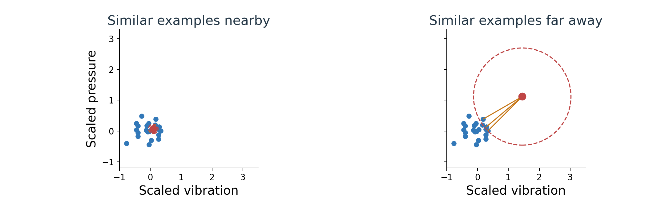
Scale features so their numerical units do not dominate distance. Choose the neighborhood and threshold using validation data. A valid new operating regime can also appear far from the existing reference.
Local density: unusual relative to nearby examples
Density describes how closely examples are packed. Local Outlier Factor (LOF) compares a point’s local density with the density around its neighbors. A valid group can be spread out, so global distance alone may not give the comparison we need.
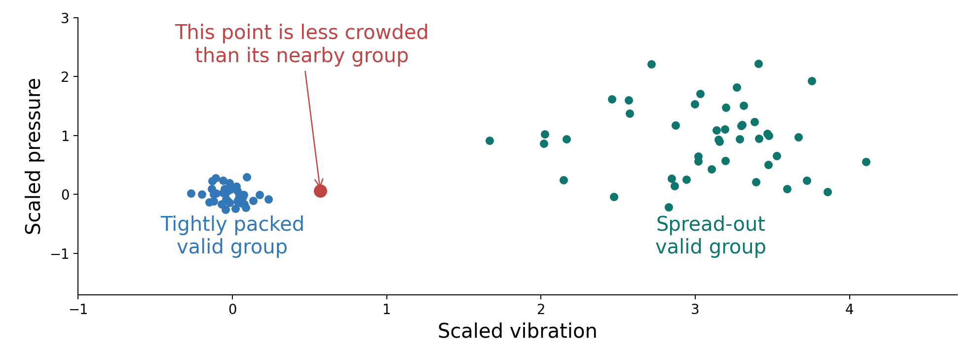
A LOF value near 1 suggests similar local density; a much larger value suggests lower local density. This ratio is further detail beyond the slide’s main idea. The figure is schematic, not a numerical LOF calculation. See Breunig et al., reference 8.
Both neighbor methods need useful features. Many irrelevant variables weaken the comparison, and temporal patterns need suitable history windows or summaries.
Isolation Forest
The question is whether a few random splits can separate an observation from the others. Isolation Forest repeatedly separates observations using random feature splits. An unusual, isolated observation often requires fewer splits than one within a large cluster. In short: the fewer cuts a point needs before it stands alone, the more unusual it is. Its anomaly score combines isolation behavior across many trees; one particular tree need not separate an anomaly quickly. See Liu et al., reference 9.
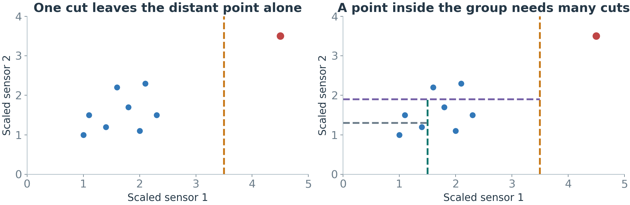
The method can work without anomaly labels, but it still needs suitable features, a threshold, and evaluation. Raw independent rows do not encode time order. Irrelevant features or a rare valid regime can also affect its scores.
Reconstruction error
The question is whether the reconstructed input differs greatly from the original. Reconstruction rebuilds an input already supplied to the model. It does not predict an unseen next reading. An autoencoder maps an input through an encoder to a compact representation, a smaller set of learned numerical features, then uses a decoder to reconstruct the input. For detection, it is often trained mainly on trusted normal examples. A sensor window that is difficult to reconstruct can receive a high anomaly score:
s(x)=\sum_j(x_j-\hat x_j)^2.
Here x_j is an input component and \hat x_j its reconstructed value. The index j can cover sensor variables, time positions, or both.
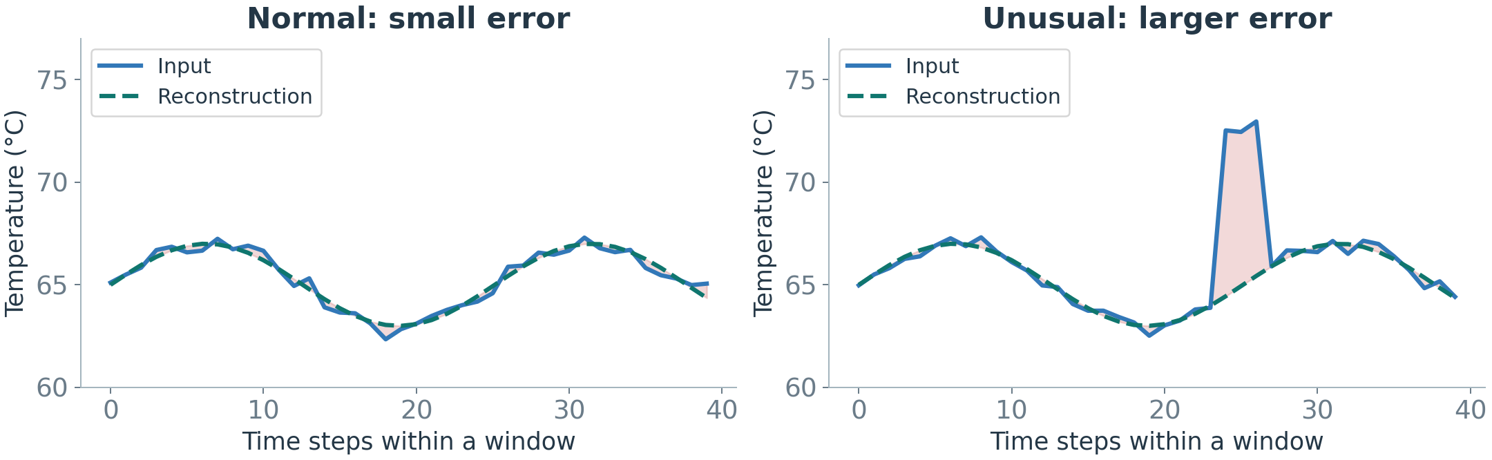
Scale inputs so one variable’s units do not dominate the error. A flexible model may also reconstruct anomalies well, especially if they appear in its training data. Large reconstruction error is evidence of a mismatch with the learned representation, not proof of a fault. Select the threshold on separate calibration or validation data.
II.D) Evaluating Anomaly Detection
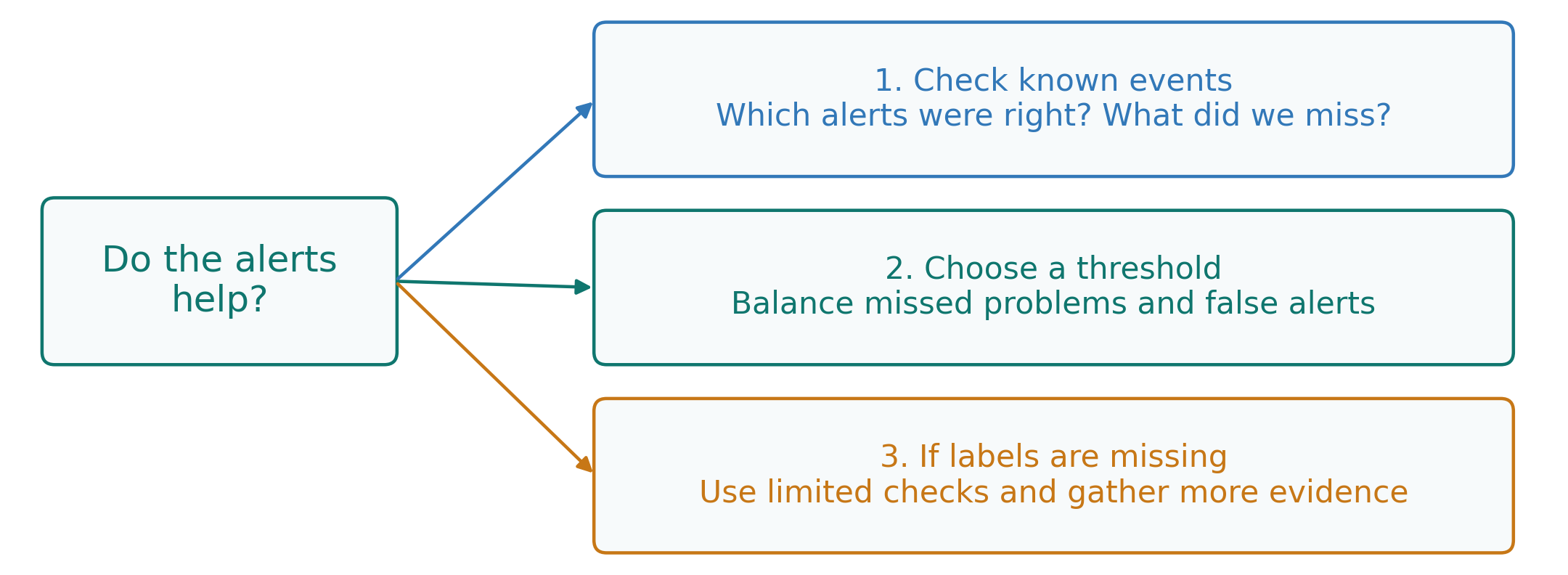
A useful detector must do more than assign scores. First check whether its alerts find independently identified anomalies. Then choose a threshold that balances missed events and false alerts. When no reliable labels exist, only more limited checks are possible.
Why accuracy alone can mislead
Suppose there are 990 normal observations and 10 anomalies. A detector that calls every observation normal achieves 990/1{,}000=99\% accuracy while detecting none of the anomalies. The dominant normal class hides complete failure at the task of interest.
Instead, count correct alerts, false alerts, and missed anomalies, and report the unit being counted.
Precision and recall, with F1 as further detail
The slide’s second example has 8 true positives (TP), 4 false positives (FP), 2 false negatives (FN), and 986 true negatives (TN). These counts refer to individual observations.
- Precision: among alerts, how many correspond to actual anomalies? P=TP/(TP+FP)=8/12=66.7\%.
- Recall: among actual anomalies, how many were detected? R=TP/(TP+FN)=8/10=80\%.
- Optional further measure, F1: the harmonic mean of precision and recall. F1=2PR/(P+R)=16/22=72.7\%.
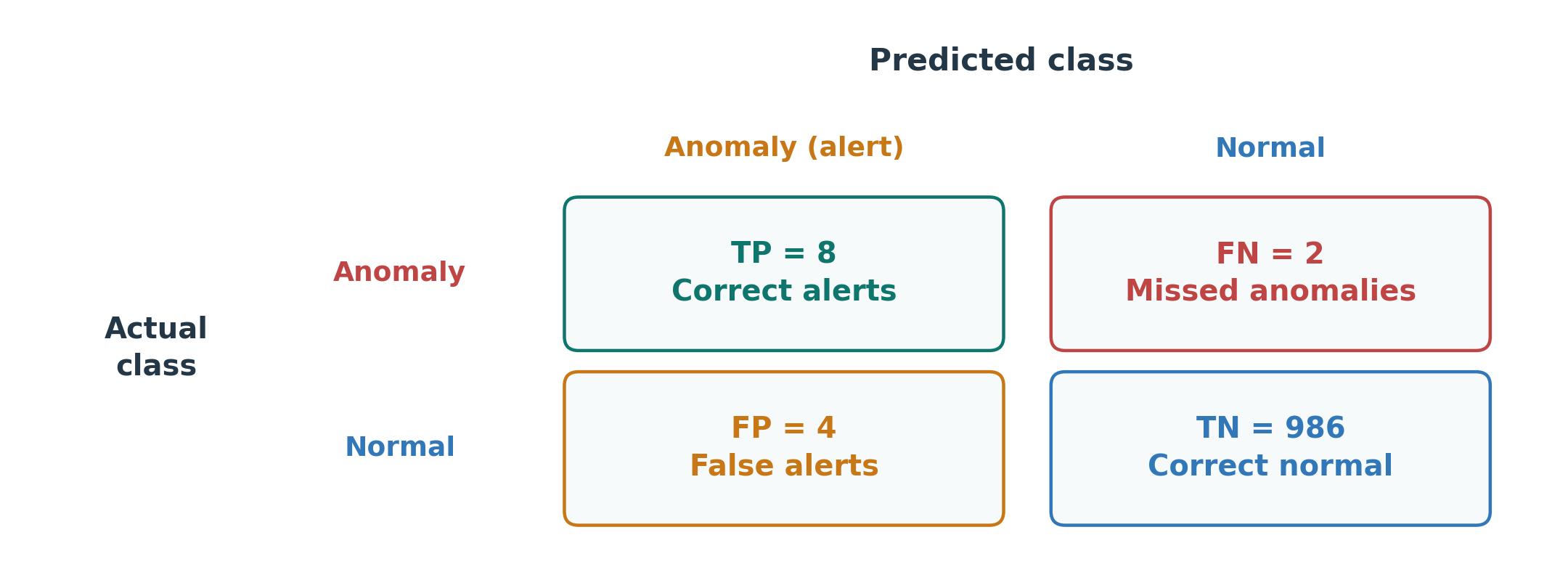
Precision describes the reliability of alerts, while recall describes the proportion of anomalies found. F1 balances the two but does not include true negatives or all operational costs. A higher F1 does not automatically imply an acceptable alert workload or response time.
Choosing a threshold
For a fixed set of scores where higher means more unusual, lowering the threshold can increase both true and false alerts. Raising it reduces alerts but may miss more events. Choose the threshold using earlier validation data and the cost of missed events, false alerts, and human review.
Without anomaly labels, a high percentile of trusted normal scores can provide an initial threshold. A percentile is a level below which a stated share of values falls: the 99th percentile is exceeded by only 1% of trusted normal scores. It gives a candidate false-alert rate under that reference, not a guarantee for future conditions. Estimating recall still requires independently identified events, including those the detector missed. Reviewing only triggered alerts cannot reveal all missed events. Never select the threshold using the final test labels.
Timestamps, incidents, and detection delay
One physical incident can span many observations. In the slide example, a fault lasts 30 readings, indexed 0 through 29, and there is exactly one alert at index 12.
- Point recall: 1/30=3.3\% of faulty timestamps are flagged.
- Event recall: 1/1=100\% of incidents are detected, if one alert within the incident counts as detection.
- Detection delay: the first alert occurs 12 sampling intervals after onset.
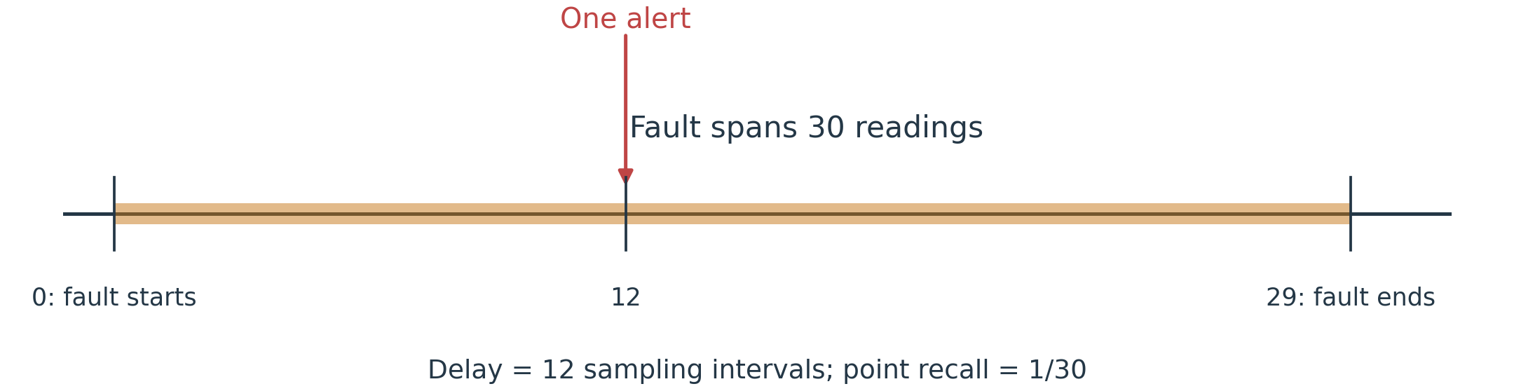
These metrics answer different questions. The event was noticed, but the alert may still be too late for the required response. If the observations are one minute apart, the delay is 12 minutes, not 12 seconds or 13 minutes.
Define incident boundaries, acceptable delay, and grouping of repeated alerts before evaluation. Report false alerts per hour as well as detection results, stating whether these are individual alert readings or grouped alarms. Do not silently count every faulty timestamp as detected because one alert occurred during the event. Clear evaluation rules matter when interpreting reported results; Sarfraz et al. discuss related evaluation problems.
Evaluation when labels are missing
The metrics above need anomaly labels for the test period. Labels for training and labels for testing are different questions: a detector trained without labels, one-class or unsupervised, should still be evaluated against a labeled test period whenever one exists, for example one built from documented past incidents.
When no labels exist at all, evaluation becomes indirect. Injected anomalies: add known artificial faults to the data and check whether the detector finds them; this tests sensitivity, but only for the fault shapes we imagine. Expert review: ask engineers to judge a sample of alerts; their verdicts become a small labeled set over time. Stability: a detector that floods operators with alerts during normal operation is not usable, whatever its potential recall. Operational usefulness: did alerts lead to findings that mattered? Treat conclusions from indirect evaluation as provisional, and record reviewed alerts so that a labeled evaluation set grows over time.
II.E) Monitoring in Practice
Operating context and changing normal behavior
Evaluation used recorded data. Once a detector runs every day, practice raises new questions, and the first is context. Expected behavior may vary with load, time of day, season, and environment. A context-aware detector compares observations with an expectation for those conditions. It can reduce false alerts caused by applying one fixed reference to several valid regimes.
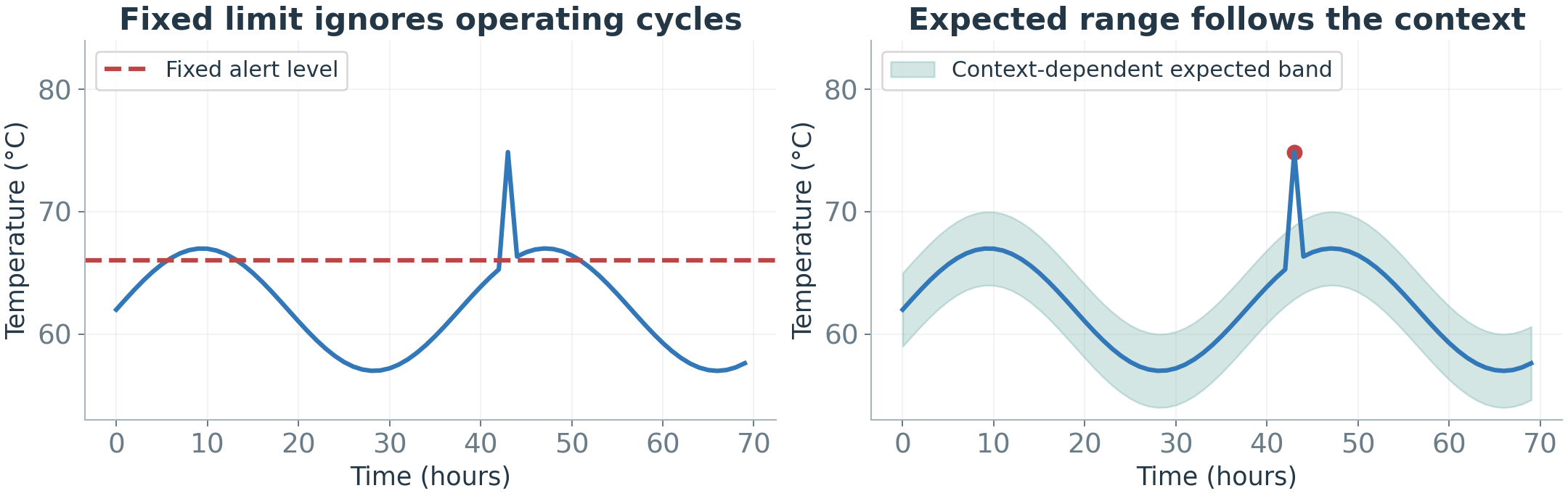
Adapt to confirmed valid changes. Keep confirmed faults out of data used to learn healthy behavior. A growing discrepancy should be investigated before being absorbed into the normal reference. Aging may explain a temperature increase without making the condition acceptable. Independent engineering limits can remain necessary even when a learned expected band changes.
Anomaly or persistent change?
A brief spike may be an isolated anomaly. A persistent deviation could reflect a valid new regime, concept drift, a sensor problem, or an ongoing fault. Duration is a clue, not a diagnosis. A fault does not become harmless because it continues for a long time.
Compare operating conditions and, where relevant, the input-to-target relationship. A shifted temperature line alone cannot distinguish changed load from altered machine behavior. Record what changed and verify its cause before updating the reference.
Online detection: checking readings as they arrive
Offline detection analyzes collected data later. Online detection evaluates a new reading or short window as it arrives. Online detection can use a fixed model; it does not require online model training.
The system must meet its response-time requirement. Window construction, waiting for several high scores, and grouping alerts can add delay. Decide how to handle late measurements and missing sensors, and use only data received by the time an alert must be issued.
Alert explanations: evidence for investigation
An engineer needs more than a score. For an alert of 0.94, show when it occurred, which conditions applied, how observed behavior differs from expected behavior, and which sensors have large discrepancies.
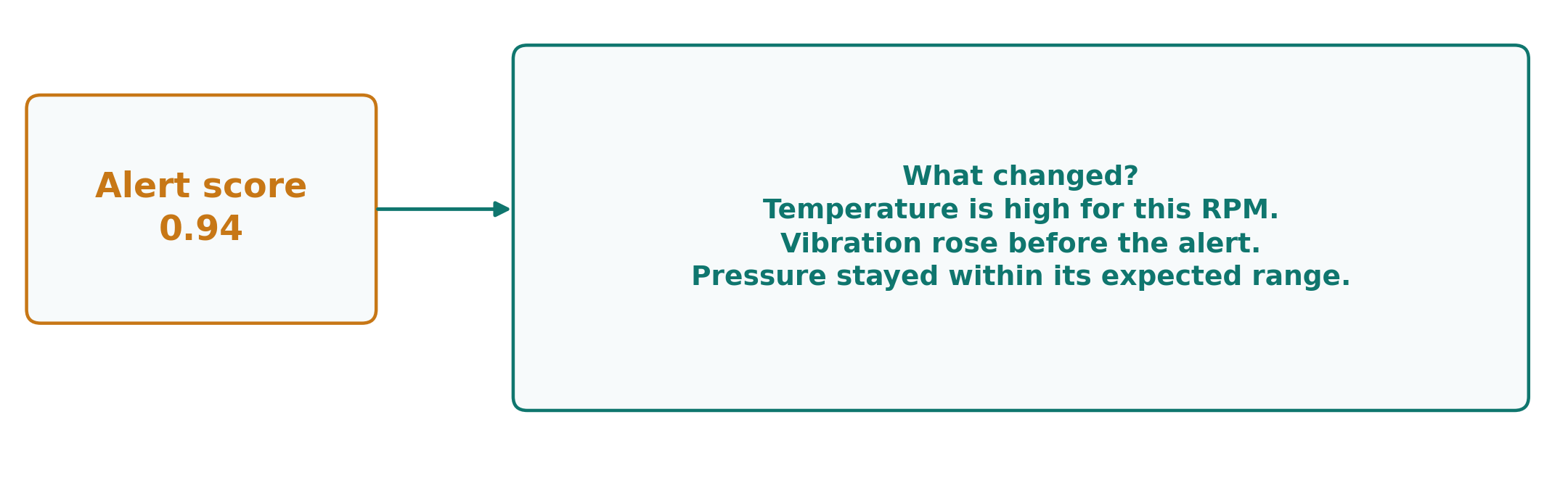
A sensor with a large discrepancy may be affected by a fault rather than its cause. An explanation guides investigation; it does not prove root cause.
Human review and controlled improvement
A reviewer checks the event and records whether it was a fault, a sensor problem, a valid event, or an unresolved case. An unreviewed alert is not a confirmed label. This feedback can improve training data and threshold selection, but changes should be explicit and validated. Keep records of the reviewed evidence and the detector version so later results can be interpreted.
II.F) From Detection to Decisions
Choosing a starting method
Choose a method from the evidence available and the type of deviation that matters. For example, known equipment limits support a rule, while a documented healthy history can support learning an expected pattern. The following table matches the slide’s starting points; it is not a ranking of algorithms.
| Available evidence | Useful starting point | Main limitation |
|---|---|---|
| Known engineering limits | Rule | Can miss context and new faults |
| Normal and fault labels | A classifier trained to distinguish the groups | May miss unfamiliar faults |
| Stable healthy readings | Statistical reference | Mixed regimes distort the reference |
| Similar normal examples | Neighbors or LOF | Scaling and neighborhood choice matter |
| Mostly normal feature vectors | Isolation Forest | Raw rows omit temporal patterns |
| Trusted normal sensor windows | Autoencoder reconstruction | Can also reconstruct anomalies |
| Reliable expected trajectory | Forecast-error score | Model errors can resemble faults |
These are possible starting points, not fixed algorithm categories. A method can be used in different learning settings depending on its training data. Whatever the starting point, compare candidate detectors on the same later data with the same incident definitions and response requirements.
Detection, diagnosis, and prognostics
These tasks ask different questions:
- Detection: does behavior differ from the expected reference?
- Diagnosis: what fault or condition is present? Root-cause analysis goes further by investigating why it occurred.
- Prognostics: how may the condition develop, or when might failure occur?
An anomaly score alone does not answer all three. Actions require additional evidence, operating constraints, and clear responsibility. These tasks are not an obligatory sequence: an urgent protective action may be needed before a full diagnosis is available.
Case study: a machine runs hotter than expected
A machine remains hotter than expected at 1,000 RPM and comparable load, while vibration also increases. Consider three questions:
- What normal reference and detector would you choose?
- Which checks could distinguish a sensor problem from physical degradation?
- What evidence would justify updating the model or healthy reference?
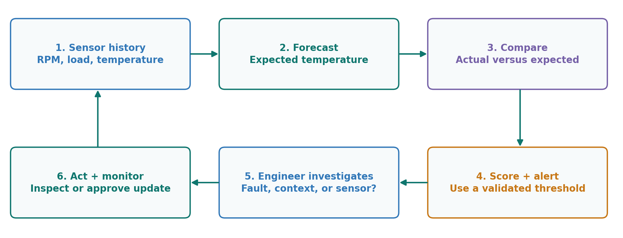
Use a documented healthy period that covers comparable RPM, load, and environment. If it supports a reliable temperature forecast, a forecast-error score is a reasonable starting point. A multivariate reference can also incorporate vibration. Choose and validate an alert threshold using earlier data.
First check timestamps, units, and calibration, and compare temperature with an independent measurement if available. Then examine vibration, maintenance history, and operating logs to see whether several signals support a physical change. These checks provide evidence; the scenario alone does not establish degradation or a particular root cause.
Update the healthy reference only after the changed behavior is confirmed to be valid for the monitoring purpose. Preserve confirmed fault examples for evaluation rather than treating them as normal. Check any proposed update on later data, and retain applicable engineering limits.
Glossary
Use this glossary to review the key terms and background vocabulary.
| Term | Definition |
|---|---|
| Time series | A sequence of observations recorded over time, in time order |
| Model | A rule or learned relationship that maps inputs to an output, such as a forecast |
| Feature / input | Information supplied to a model, such as past readings or load |
| Target | The value the model tries to predict |
| Training | Adjusting a model using training data; the forecasting examples here pair past inputs with known future outcomes |
| Prediction | Applying a model to estimate an outcome that is not yet known |
| Baseline | A simple comparison method used to judge whether another method adds value |
| Decomposition | Separating an observed series into estimated components, here trend plus seasonality plus remainder |
| Trend | The underlying level and longer-term direction of a series |
| Seasonality | Variation that repeats at a regular interval, such as a daily cycle |
| Remainder | What is left after subtracting the estimated trend and seasonality; not necessarily random noise |
| Lag | A time offset from a stated reference time; for forecasting here, lag 1 is the reading one step before the target |
| Autocorrelation | The linear relationship between readings of the same series at a chosen lag |
| Temporal dependence | A statistical relationship between observations made at different times |
| Stationarity (weak) | A constant mean and spread, with linear dependence depending on the time gap rather than the date |
| Variance | A measure of spread: the average squared distance of values from their mean; the standard deviation is its square root |
| Differencing | Replacing a series by the change between consecutive readings, which can reduce a trend |
| Forecast origin | The moment a forecast is made; only information available then may be used |
| Lookback window | The span of history supplied to a forecasting model |
| Forecast horizon | How far ahead a forecast reaches |
| Covariate | A related input variable added to a forecast, such as RPM or a known future load schedule |
| Naive forecast | Repeat the latest observed value; the seasonal version repeats the value from the last cycle |
| Exponential smoothing | Updating an estimated level by blending the newest reading with the previous level using a weight alpha |
| ARIMA | A statistical model combining past values (AR), differencing (I), and past forecast errors (MA) |
| Linear regression | A model that predicts a target as a weighted sum of input features plus a constant |
| Decision tree | A model made of learned if-then splits on feature values that lead to a prediction |
| Random forest | An ensemble that averages the predictions of many decision trees |
| Gradient boosting | An ensemble that adds decision trees one at a time, each correcting the remaining error |
| Ensemble | Any model that combines the predictions of several models |
| Sequence model | A neural model that reads an ordered history, such as a recurrent network |
| LSTM | Long short-term memory: a recurrent network using gates to control what information is retained |
| Convolution (temporal) | Sliding a small learned pattern template, called a filter, across neighboring time steps |
| Attention | A mechanism that learns how much information to draw from each observed position |
| Transformer | A neural architecture built around attention, used by some forecasting models |
| Foundation model (time series) | A model pretrained on many series that can be applied or adapted to new ones |
| Zero-shot forecasting | Applying a pretrained model to a new series without updating its weights on that series |
| Prediction interval | A range expressing uncertainty about a future observation; not a safe operating range |
| Coverage | The share of evaluated observations that fall inside their prediction intervals |
| MAE, RMSE, MAPE | Mean absolute error; root mean squared error, which weights large errors more; mean absolute percentage error |
| Temporal split | Training on the past and evaluating on a later period, in time order |
| Walk-forward validation | Repeating forecasting at successive origins, fitting only on data available at each origin |
| Data leakage | Using information in training or features that was not available at the forecast origin |
| Scaler | A preprocessing step that adjusts feature ranges; fit it on training data only |
| Distribution | How values of a quantity are spread across their possible range |
| Covariate shift | The input conditions change while the input-target relationship stays the same; also called virtual drift |
| Concept drift | The input-target relationship itself changes; also called real drift |
| Model degradation | Predictive performance becoming worse over time after deployment |
| Online learning | Updating a model incrementally as new training data arrive |
| Anomaly | An observation or pattern that differs meaningfully from expected behavior |
| Normal reference | The evidence used to describe expected behavior for a task and operating conditions |
| Point, contextual, collective anomaly | Unusual alone; unusual for its time or condition; an unusual pattern across several readings |
| One-class setting | Training mainly on trusted normal examples to learn the boundary of normal behavior |
| z-score | Distance from a reference mean measured in standard deviations |
| Skewed data | A lopsided distribution with a longer tail on one side, which can distort a single mean and spread |
| Percentile | A level below which a stated share of values falls; the 99th percentile is exceeded by 1% of values |
| kNN detection | Here, scoring an observation by its distance to the kth nearest reference point |
| Local Outlier Factor (LOF) | Comparing an observation’s local density with its neighbors’ density; a value near 1 indicates similar local density |
| Density (local) | How crowded the reference examples are in the neighborhood of a point |
| Isolation Forest | Scoring by how few random splits are needed to separate an observation |
| Multivariate detection | Examining several measurements and their relationships to identify unusual combinations |
| Anomaly score | A measure of how unusual an observation appears under a detector; not automatically a probability |
| Reconstruction error | The difference between an input and its reconstruction by a model such as an autoencoder |
| Threshold | The score level above which an alert is raised |
| Precision | The share of alerts that are correct: TP / (TP + FP) |
| Recall | The share of true anomalies that are found: TP / (TP + FN) |
| F1 score | The harmonic combination of precision and recall: 2PR / (P + R) |
| Event recall | The share of whole incidents detected at least once, as opposed to counting timestamps |
| Detection delay | How long after an incident begins the first alert occurs |
| Online detection | Scoring each new reading as it arrives, which need not involve online training |
Week 4 Summary
Forecasting estimates what should happen next. Anomaly detection compares observed behavior with an appropriate expectation. In both tasks, the value of a result depends on the information available, the evaluation design, and the decision it supports.
Before applying the methods, be able to explain:
- What is observed, what must be predicted or detected, and which information is available at that time?
- Which baseline or normal reference provides a meaningful comparison?
- Does evaluation follow time and avoid future information?
- Are uncertainty, thresholds, missed events, false alerts, and delay measured appropriately?
- What evidence is needed to investigate a change and decide whether to update the model?
For further reading, use the references on the Week 4 page. The slides provide the accompanying presentation figures and examples.